User guide
Rings library structure
Rings has the following main components:
rings.bigint
arbitrary precision integers (fork of tbuktu/bigint)rings.primes
prime numbers including prime factorization, primality test etc.rings.poly.univar
univariate polynomials and algorithms with them including GCD and factorizationrings.poly.multivar
multivariate polynomials and algorithms with them including GCD, factorization, Gröbner basis etc.rings.io
methods for parsing/stringifying mathematical expressionsrings.scaladsl
Scala wrappers and syntax definitions for Rings
Examples in this user guide require some imports to be in the scope. The following code snippet includes all possible imports that may be required to run examples:
import cc.redberry.rings
import rings.{bigint, primes, poly}
import rings.poly.{univar, multivar}
import rings.scaladsl._
import syntax._
import cc.redberry.rings.*
import cc.redberry.rings.poly.*
import cc.redberry.rings.poly.univar.*
import cc.redberry.rings.poly.multivar.*

import static cc.redberry.rings.poly.PolynomialMethods.*
import static cc.redberry.rings.Rings.*
Numbers
Integers
There are two basic types of integer numbers that we have to deal with when doing algebra in computer: machine integers and arbitrary-precision integers. For the machine integers the Java’s primitive 64-bit long type is used (since most modern CPUs are 64-bit). Internally Rings uses machine numbers for representation of integers modulo prime numbers less than \(2^{64}\) which is done for performance reasons (see Modular arithmetic with machine integers). For the arbitrary-precision integers Rings uses improved BigInteger class github.com/tbuktu/bigint (rings.bigint.BigInteger) instead of built-in java.math.BigInteger. The improved BigInteger has Schönhage-Strassen multiplication and Barrett division algorithms for large integers which is a significant performance improvement in comparison to native Java’s implementation.
Tip
In order to avoid confusing of BigInteger used in Rings and java.math.BigInteger it is convenient to instantiate arbitrary-precision integers via methods provided in ring Z.
In Java:
BigInteger fromString = Z.parse("12345689");
BigInteger fromInt    = Z.valueOf(12345689);
BigInteger fromLong   = Z.valueOf(1234568987654321L);
In Scala:
val fromString : IntZ = Z("12345689")
val fromInt    : IntZ = Z(12345689)
val fromLong   : IntZ = Z(1234568987654321L)
(the type definition type IntZ = ring.bigint.BigInteger is introduced in Scala DSL)
Prime numbers
In many applications it is necessary to test primality of integer number (isPrime(number)) or to generate some prime numbers (nextPrime(number)). This is realized in the following two classes:
- SmallPrimes for numbers less than \(2^{32}\). It uses Miller-Rabin probabilistic primality test for int type in such a way that result is always guaranteed (code is adapted from Apache Commons Math).
- BigPrimes for arbitrary large numbers. It switches between Pollard-Rho, Pollard-P1 and Quadratic Sieve algorithms for prime factorization and also uses probabilistic Miller-Rabin test and strong Lucas test for primality testing.
The following code snippet gives some illustrations:
int intNumber = 1234567;
// false
boolean primeQ = SmallPrimes.isPrime(intNumber);
// 1234577
int intPrime = SmallPrimes.nextPrime(intNumber);
// [127, 9721]
int[] intFactors = SmallPrimes.primeFactors(intNumber);

long longNumber = 12345671234567123L;
// false
primeQ = BigPrimes.isPrime(longNumber);
// 12345671234567149
long longPrime = BigPrimes.nextPrime(longNumber);
// [1323599, 9327350077]
long[] longFactors = BigPrimes.primeFactors(longNumber);

BigInteger bigNumber = Z.parse("321536584276145124691487234561832756183746531874567");
// false
primeQ = BigPrimes.isPrime(bigNumber);
// 321536584276145124691487234561832756183746531874827
BigInteger bigPrime = BigPrimes.nextPrime(bigNumber);
// [3, 29, 191, 797359, 1579057, 14916359, 1030298906727233717673336103]
List<BigInteger> bigFactors = BigPrimes.primeFactors(bigNumber);
Modular arithmetic with machine integers
One important implementation aspect concerns arithmetic in the ring \(Z_p\) with \(p < 2^{64}\), that is integer arithmetic modulo some machine number. Though it may be hidden from the user’s eye, arithmetic in this ring actually lies in the basis of the most part of fundamental algorithms and directly affects performance of nearly all computations. In contrast to \(Z_p\) with arbitrary large characteristic, for characteristic that fits into 64-bit word one can use machine integers to significantly speed up basic math operations. On the CPU level the modulo operation is implemented via DIV instruction (integer division) which is known to be very slow: for example on the recent Intel Skylake architecture DIV has 20-80 times worse throughput than MUL instruction (see this report). Hopefully, arithmetic operations in \(Z_p\) are done modulo a fixed modulus \(p\) which allows to make some preconditioning on \(p\) and reduce DIV operations to MUL. The idea is the following: given a fixed \(p\) we compute once the value of \(magic = [2^n/p]\) with a sufficiently large \(n\) (so that magic is some non-zero machine number), and then for arbitrary integer \(a\) we have \([a/p] = (a \times magic)/2^n\), so DIV instruction is replaced with one MUL and one SHIFT (division by a power of two is just a bitwise shift, very fast). The actual implementation in fact requires some more work to do (for details see Chapter 10 in Hacker’s Delight). Rings uses libdivide4j library for fast integer division with precomputation which is ported from the well known C/C++ libdivide library. With this precomputation the mod operation becomes several times faster than the native CPU instruction, which boosts the overall performance of many of Rings algorithms in more than 3 times.
The ring \(Z_p\) with \(p < 2^{64}\) is implemented in IntegersZp64 class (while IntegersZp implements \(Z_p\) with arbitrary large characteristic). IntegersZp64 defines all arithmetic operations in \(Z_p\):
// Z/p with p = 2^7 - 1 (Mersenne prime)
IntegersZp64 field = new IntegersZp64(127);
//     1000 = 111 mod 127
assert field.modulus(1000) == 111;
// 100 + 100 = 73 mod 127
assert field.add(100, 100) == 73;
//  12 - 100 = 39 mod 127
assert field.subtract(12, 100) == 39;
//  55 * 78  = 73 mod 127
assert field.multiply(55, 78) == 99;
//   1 / 43  = 65 mod 127
assert field.reciprocal(43) == 65;
It is worst to mention, that multiplication defined in IntegersZp64 is especially fast when characteristic is less than \(2^{32}\): in this case multiplication of two numbers fits the machine 64-bit word (no long overflow), while in the opposite case Montgomery reduction will be used:
// Z/p with p = 2^31 - 1 (Mersenne prime) - fits 32-bit word
IntegersZp64 field32 = new IntegersZp64((1L << 31) - 1L);
// does not cause long overflow - fast
assert field32.multiply(0xabcdef12, 0x12345678) == 0x7e86a4d6;


// Z/p with p = 2^61 - 1 (Mersenne prime) - doesn't fit 32-bit word
IntegersZp64 field64 = new IntegersZp64((1L << 61) - 1L);
// cause long overflow - Montgomery reduction will be used - not so fast
assert field64.multiply(0x0bcdef1234567890L, 0x0234567890abcdefL) == 0xf667077306fd7a8L;
Note
IntegersZp64 is used in order to achieve the best possible performance of many fundamental algorithms which underlie in the basis of many high-level features such as GCD and factorization in arbitrary polynomial rings. Since IntegersZp64 operates with primitive longs and Java doesn’t support generics with primitives, IntegersZp64 stands separately from the elegant type hierarchy of generic rings implemented in Rings (see Rings). For the same reason some of the algorithms have two implementations: one for rings over generic elements and one for IntegersZp64. This internal complication is hidden from the user, and the switch between generic and primitive types is done automatically in the internals of Rings when it can really make gain in the performance.
Rings
The concept of mathematical ring is implemented in the generic interface Ring<E> which defines all basic algebraic operations over the elements of type E. The simplest example is the ring of integers \(Z\) (Z), which operates with Rings BigInteger instances and simply delegates all operations like + or * to methods of class BigInteger. A little bit more complicated ring is a ring of integers modulo some number (\(Z_p\)):
// The ring Z/17
Ring<BigInteger> ring = Zp(Z.valueOf(17));

//     103 = 1 mod 17
BigInteger el  = ring.valueOf(Z.valueOf(103));
assert  el.intValue() == 1;

// 99 + 88 = 0 mod 17
BigInteger add = ring.add(Z.valueOf(99),
                          Z.valueOf(88));
assert add.intValue() == 0;

// 99 * 77 = 7 mod 17
BigInteger mul = ring.multiply(Z.valueOf(99),
                               Z.valueOf(77));
assert mul.intValue() == 7;

// 1  / 99 = 11 mod 17
BigInteger inv = ring.reciprocal(Z.valueOf(99));
assert inv.intValue() == 11;
The interface Ring<E> additionally defines algebraic operations inherent to more specialized types of rings:
- GCD domains
rings that support GCD operation- Euclidean rings
rings that support division with remainder- Fields
rings that support exact division
These operations can be summarized in the following methods from Ring<E> interface:
// Methods from Ring<E> interface:

// GCD domain operation:
E gcd(E a, E b);

// Euclidean ring operation:
E[] divideAndRemainder(E dividend, E divider);

// Field operation:
E reciprocal(E element);
One can check whether the ring R is a field or a Euclidean ring using R.isField() and R.isEuclideanRing() methods.
Important
If one invoke field method like reciprocal(el) on a ring which is not a field, the UnsupportedOperationException will be thrown:
// ring Z
Ring<BigInteger> notField = Z;
// it is not a fielf
assert !notField.isField();
// this is OK (1/1 = 1)
assert notField.reciprocal(Z.getOne()).isOne();
// this will throw UnsupportedOperationException
notField.reciprocal(Z.valueOf(10)); // <- error
Each Ring<E> implementation provides the information about its mathematical nature and its properties like cardinality, characteristic etc. Another important method defined in Ring<E> is parse(String) which converts string into ring element. Illustrations:
// Z is not a field
assert  Z.isEuclideanRing();
assert !Z.isField();
assert !Z.isFinite();

// Q is an infinite field
assert  Q.isField();
assert !Q.isFinite();
assert  Q.parse("2/3").equals(
       new Rational<>(Z, Z.valueOf(2), Z.valueOf(3)));

// GF(2^10) is a finite field
FiniteField<UnivariatePolynomialZp64> gf = GF(2, 10);
assert gf.isField();
assert gf.isFinite();
assert gf.characteristic().intValue() == 2;
assert gf.cardinality().intValue() == 1 << 10;
System.out.println(gf.parse("1 + z + z^10"));

// Z/3[x] is Euclidean ring but not a field
UnivariateRing<UnivariatePolynomialZp64> zp3x = UnivariateRingZp64(3);
assert  zp3x.isEuclideanRing();
assert !zp3x.isField();
assert !zp3x.isFinite();
assert  zp3x.characteristic().intValue() == 3;
assert  zp3x.parse("1 + 14*x + 15*x^10").equals(
       UnivariatePolynomialZ64.create(1, 2).modulus(3));
Finally, each Ring<E> implementation provides a set of high-level methods for GCDs, factorization etc. Below is the summary of main Ring<E> methods:
| Method from Ring<E> | Description |
|---|---|
add(a, b) |
Ring addition |
subtract(a, b) |
Ring subtraction |
multiply(a, b) |
Ring multiplication |
isEuclideanRing() |
Whether ring supports division with remainder |
divideAndRemainder(a, b) |
Division with remainder (for Euclidean rings) |
isField() |
Whether ring is a field |
reciprocal(a) |
Multiplicative inverse (for fields) |
getOne() |
Identity element under multiplication |
getZero() |
Identity element under addition |
characteristic() |
Ring characteristic |
cardinality() |
Ring cardinality |
parse(string) |
Parse ring element from string |
randomElement() |
Pick some random ring element |
gcd(a, b) |
Greatest common divisor of two elements |
factor(a) |
Unique factor decomposition of ring element |
factorSquareFree(a) |
Square free decomposition of ring element |
The full list of Ring<E> methods can be found in corresponding Java docs
List of built-in rings
Basic rings and factory methods for constructing new rings are placed in Rings class (Java) or directly in scaladsl package object (Scala). Below is the list of what is available by default in Rings:
| Ring | Description | Method in Rings / scaladsl |
|---|---|---|
| \(Z\) | Ring of integers | Z |
| \(Q\) | Field of rationals | Q |
| \(Z_p\) | Integers modulo \(p\) | Zp(p) |
| \(Z_p\) with \(p < 2^{64}\) | Integers modulo \(p < 2^{64}\) | Zp64(p) [*] |
| \(GF(p^q)\) | Galois field with cardinality \(p^q\) | GF(p, q) and GF(irred) or GF(p, q, var) and GF(irred, var) in Scala |
| \(Frac(R)\) | Field of fractions of an integral domain \(R\) | Frac(R) |
| \(R[x]\) | Univariate polynomial ring over coefficient ring \(R\) | UnivariateRing(R) or UnivariateRing(R, var) in Scala |
| \(Z_p[x]\) with \(p < 2^{64}\) | Univariate polynomial ring over coefficient ring \(Z_p\) with \(p < 2^{64}\) | UnivariateRingZp64(p) or UnivariateRingZp64(p, var) in Scala |
| \(R[x_1, \dots, x_N]\) | Multivariate polynomial ring with exactly \(N\) variables over coefficient ring \(R\) | MultivariateRing(N, R) or MultivariateRing(R, vars) in Scala |
| \(Z_p[x_1, \dots, x_N]\) with \(p < 2^{64}\) | Multivariate polynomial ring with exactly \(N\) variables over coefficient ring \(Z_p\) with \(p < 2^{64}\) | MultivariateRingZp64(N, p) or MultivariateRingZp64(p, vars) in Scala |
| \(R[x]/\langle p(x) \rangle\) | Univariate quotient ring | UnivariateQuotientRing(baseRing, poly) |
| \(R[x_1, \dots, x_N]/I\) | Multivariate quotient ring | QuotientRing(baseRing, ideal) |
| [*] | Class IntegersZp64 which represents \(Z_p\) with \(p < 2^{64}\) does not inherit Ring<E> interface (see Modular arithmetic with machine integers) |
Galois fields
Galois field \(GF(p^q)\) with prime characteristic \(p\) and cardinality \(p^q\) can be created by specifying \(p\) and \(q\) in which case the irreducible polynomial will be generated automatically or by explicitly specifying the irreducible:
// Galois field GF(7^10) represented by univariate polynomials
// in variable "z" over Z/7 modulo some irreducible polynomial
// (irreducible polynomial will be generated automatically)
val gf7_10 = GF(7, 10, "z")
assert(gf7_10.characteristic == Z(7))
assert(gf7_10.cardinality == Z(7).pow(10))

// GF(7^3) generated by irreducible polynomial "1 + 3*z + z^2 + z^3"
val gf7_3 = GF(UnivariateRingZp64(7, "z")("1 + 3*z + z^2 + z^3"), "z")
assert(gf7_3.characteristic == Z(7))
assert(gf7_3.cardinality == Z(7 * 7 * 7))
// Galois field GF(7^10)
// (irreducible polynomial will be generated automatically)
FiniteField<UnivariatePolynomialZp64> gf7_10 = GF(7, 10);
assert gf7_10.characteristic().intValue() == 7;
assert gf7_10.cardinality().equals(Z.valueOf(7).pow(10));

// GF(7^3) generated by irreducible polynomial "1 + 3*z + z^2 + z^3"
FiniteField<UnivariatePolynomialZp64> gf7_3 = GF(UnivariatePolynomialZ64.create(1, 3, 1, 1).modulus(7));
assert gf7_3.characteristic().intValue() == 7;
assert gf7_3.cardinality().intValue() == 7 * 7 * 7;
Galois fields with arbitrary large characteristic are available:
// Mersenne prime 2^107 - 1
val characteristic = Z(2).pow(107) - 1
// Galois field GF((2^107 - 1) ^ 16)
implicit val field = GF(characteristic, 16, "z")

assert(field.cardinality() == characteristic.pow(16))
// Mersenne prime 2^107 - 1
BigInteger characteristic = Z.getOne().shiftLeft(107).decrement();
// Galois field GF((2^107 - 1) ^ 16)
FiniteField<UnivariatePolynomial<BigInteger>> field = GF(characteristic, 16);

assert(field.cardinality().equals(characteristic.pow(16)));
Implementation of Galois fields uses assymptotically fast algorithm for polynomial division with precomputed inverses via Newton iterations (see Univariate division with remainder).
Fields of fractions
Field of fractions can be defined over any GCD ring \(R\). The simplest example is the field \(Q\) of fractions over \(Z\):
implicit val field = Frac(Z) // the same as Q

assert( field("13/6") == field("2/3") + field("3/2") )
assert( field("5/6")  == field("2/3") + field("1/6") )
Rationals<BigInteger> field = Frac(Z); // the same as Q

assert field.parse("13/6")
        .equals(field.add(field.parse("2/3"),
                field.parse("3/2")));

assert field.parse("5/6")
        .equals(field.add(
                field.parse("2/3"),
                field.parse("1/6")));
The common GCD is automatically canceled in the numerator and denominator. Another illustration: field \(Frac(Z[x, y, z])\) of rational functions over \(x\), \(y\) and \(z\):
val ring = MultivariateRing(Z, Array("x", "y", "z"))
implicit val field = Frac(ring)

val a = field("(x + y + z)/(1 - x - y)")
val b = field("(x^2 - y^2 + z^2)/(1 - x^2 - 2*x*y - y^2)")

println(a + b)
Ring<MultivariatePolynomial<BigInteger>> ring = MultivariateRing(3, Z);
Ring<Rational<MultivariatePolynomial<BigInteger>>> field = Frac(ring);

Rational<MultivariatePolynomial<BigInteger>>
        a = field.parse("(x + y + z)/(1 - x - y)"),
        b = field.parse("(x^2 - y^2 + z^2)/(1 - x^2 - 2*x*y - y^2)");

System.out.println(field.add(a, b));
Rational function arithmetic
Since it is often used in practice, it is worth to put examples with the field of rational functions in a separate section, though this is just a particular case of generic field of fractions. Field of rational functions is defined as \(Frac(Z[\vec X])\). The below example llustrates how to parse elements of the field \(Frac(Z[x,y,z])\) from strings, do basic and advanced math operations in it:
// Frac(Z[x,y,z])
implicit val field = Frac(MultivariateRing(Z, Array("x", "y", "z")))

// parse some math expression from string
// it will be automatically reduced to a common denominator
// with the gcd being automatically cancelled
val expr1 = field("(x/y/(x - z) + (x + z)/(y - z))^2 - 1")

// do some math ops programmatically
val (x, y, z) = field("x", "y", "z")
val expr2 = expr1.pow(2) + x / y - z

// bind expr1 and expr2 to variables to use them further in parser
field.coder.bind("expr1", expr1)
field.coder.bind("expr2", expr2)

// parse some complicated expression from string
// it will be automatically reduced to a common denominator
// with the gcd being automatically cancelled
val expr3 = field(
  """
     expr1 / expr2 - (x*y - z)/(x-y)/expr1
     + x / expr2 - (x*z - y)/(x-y)/expr1/expr2
     + x^2*y^2 - z^3 * (x - y)^2
  """)

// export expression to string
println(field.stringify(expr3))

// take numerator and denominator
val num = expr3.numerator()
val den = expr3.denominator()
// common GCD is always cancelled automatically
assert( field.ring.gcd(num, den).isOne )

// compute unique factor decomposition of expression
val factors = field.factor(expr3)
println(field.stringify(factors))
MultivariateRing<MultivariatePolynomial<BigInteger>> ring = MultivariateRing(3, Z);
Rationals<MultivariatePolynomial<BigInteger>> field = Frac(ring);

// Parser/stringifier of rational functions
Coder<Rational<MultivariatePolynomial<BigInteger>>, ?, ?> coder
     = Coder.mkRationalsCoder(
            field,
            Coder.mkMultivariateCoder(ring, "x", "y", "z"));

// parse some math expression from string
// it will be automatically reduced to a common denominator
// with the gcd being automatically cancelled
Rational<MultivariatePolynomial<BigInteger>> expr1 = coder.parse("(x/y/(x - z) + (x + z)/(y - z))^2 - 1");

// do some math ops programmatically
Rational<MultivariatePolynomial<BigInteger>>
x = new Rational<>(ring, ring.variable(0)),
y = new Rational<>(ring, ring.variable(1)),
z = new Rational<>(ring, ring.variable(2));

Rational<MultivariatePolynomial<BigInteger>> expr2 = field.add(
        field.pow(expr1, 2),
        field.divideExact(x, y),
        field.negate(z));


// bind expr1 and expr2 to variables to use them further in parser
coder.bind("expr1", expr1);
coder.bind("expr2", expr2);

// parse some complicated expression from string
// it will be automatically reduced to a common denominator
// with the gcd being automatically cancelled
Rational<MultivariatePolynomial<BigInteger>> expr3 = coder.parse(
          " expr1 / expr2 - (x*y - z)/(x-y)/expr1"
        + " + x / expr2 - (x*z - y)/(x-y)/expr1/expr2"
        + "+ x^2*y^2 - z^3 * (x - y)^2");

// export expression to string
System.out.println(coder.stringify(expr3));

// take numerator and denominator
MultivariatePolynomial<BigInteger> num = expr3.numerator();
MultivariatePolynomial<BigInteger> den = expr3.denominator();

// common GCD is always cancelled automatically
assert field.ring.gcd(num, den).isOne();

// compute unique factor decomposition of expression
FactorDecomposition<Rational<MultivariatePolynomial<BigInteger>>> factors = field.factor(expr3);
System.out.println(factors.toString(coder));
Tip
One can use both \(Frac(Z[\vec X])\) and \(Frac(Q[\vec X])\) to represent field of rational functions. In the latter case, numeric denominators will be absorbed in polynomial coefficients, while in the former the common numeric denominator will be always factored out (so all polynomials will have only integer coefficients). From the mathematical point of view, there is no difference, while from the implementation point of view arithmetic in \(Frac(Z[\vec X])\) will be always faster since it avoids unnecessary conversions from \(Q[\vec X]\) to \(Z[\vec X]\) performed internally in GCD algorithms.
Univariate polynomial rings
Polynomial ring \(R[x]\) can be defined over arbitrary coefficient ring \(R\). There are two separate implementations of univariate rings:
UnivariateRingZp64(p)
Ring of univariate polynomials over \(Z_p\) with \(p < 2^{64}\). Implementation of this ring uses specifically optimized data structures and efficient algorithms for arithmetic in \(Z_p\) (see Modular arithmetic with machine integers).UnivariateRing(R)
Ring of univariate polynomials over generic coefficient domain \(R\).
Illustrations:
// Ring Z/3[x]
val zp3x = UnivariateRingZp64(3, "x")
// parse univariate poly from string
val p1 = zp3x("4 + 8*x + 13*x^2")
val p2 = zp3x("4 - 8*x + 13*x^2")
assert (p1 + p2 == zp3x("2 - x^2") )


// GF(7^3)
val cfRing = GF(UnivariateRingZp64(7, "z")("1 + 3*z + z^2 + z^3"), "z")
// GF(7^3)[x]
val gfx = UnivariateRing(cfRing, "x")
// parse univariate poly from string
val r1 = gfx("4 + (8 + z)*x + (13 - z^43)*x^2")
val r2 = gfx("4 - (8 + z)*x + (13 + z^43)*x^2")
assert(r1 + r2 == gfx("1 - 2*x^2"))
val (div, rem) = r1 /% r2
assert(r1 == r2 * div + rem)
// Ring Z/3[x]
UnivariateRing<UnivariatePolynomialZp64> zp3x = UnivariateRingZp64(3);
// parse univariate poly from string
UnivariatePolynomialZp64
        p1 = zp3x.parse("4 + 8*x + 13*x^2"),
        p2 = zp3x.parse("4 - 8*x + 13*x^2");
assert zp3x.add(p1, p2).equals(zp3x.parse("2 - x^2"));


// GF(7^3)
FiniteField<UnivariatePolynomialZp64> cfRing = GF(UnivariateRingZp64(7).parse("1 + 3*z + z^2 + z^3"));
// GF(7^3)[x]
UnivariateRing<UnivariatePolynomial<UnivariatePolynomialZp64>> gfx = UnivariateRing(cfRing);
// parse univariate poly from string
UnivariatePolynomial<UnivariatePolynomialZp64>
        r1 = gfx.parse("4 + (8 + z)*x + (13 - z^43)*x^2"),
        r2 = gfx.parse("4 - (8 + z)*x + (13 + z^43)*x^2");
assert gfx.add(r1, r2).equals(gfx.parse("1 - 2*x^2"));
UnivariatePolynomial<UnivariatePolynomialZp64>
        divRem[] = divideAndRemainder(r1, r2),
        div = divRem[0],
        rem = divRem[1];
assert r1.equals(gfx.add(gfx.multiply(r2, div), rem));
Tip
For univariate polynomial rings over \(Z_p\) with \(p < 2^{64}\) it is always preferred to use UnivariateRingZp64(p, "x") instead of generic UnivariateRing(Zp(p), "x"). In the latter case the generic data structures will be used (arbitrary precision integers etc.), while in the former the specialized implementation and algorithms will be used (see Modular arithmetic with machine integers) which are in several times faster than the generic ones. For example, from the mathematical point of view the following two lines define the same ring \(Z_{3}[x]\):
val ringA = UnivariateRingZp64(3, "x")
val ringB = UnivariateRing(Zp(3), "x")
Though the math meaning is the same, ringA uses optimized polynomials UnivariatePolynomialZp64 while ringB uses generic UnivariatePolynomial<E>; as result, operations in ringA are in several times faster than in ringB.
Further details about univariate polynomials are in Univariate polynomials section.
Multivariate polynomial rings
Polynomial ring \(R[x_1, \dots, x_N]\) can be defined over arbitrary coefficient ring \(R\). There are two separate implementations of multivariate rings:
MultivariateRingZp64(N, p)
Ring of multivariate polynomials with exactly \(N\) variables over \(Z_p\) with \(p < 2^{64}\). Implementation of this ring uses specifically optimized data structures and efficient algorithms for arithmetic in \(Z_p\) (see Modular arithmetic with machine integers).MultivariateRing(N, R)
Ring of multivariate polynomials with exactly \(N\) variables over generic coefficient domain \(R\).
Illustrations:
// Ring Z/3[x, y, z]
val zp3xyz = MultivariateRingZp64(3, Array("x", "y", "z"))
// parse univariate poly from string
val p1 = zp3xyz("4 + 8*x*y + 13*x^2*z^5")
val p2 = zp3xyz("4 - 8*x*y + 13*x^2*z^5")
assert (p1 + p2 == zp3xyz("2 - x^2*z^5") )


// GF(7^3)
val cfRing = GF(UnivariateRingZp64(7, "t")("1 + 3*t + t^2 + t^3"), "t")
// GF(7^3)[x, y, z]
val gfx = MultivariateRing(cfRing, Array("x", "y", "z"))
// parse univariate poly from string
val r1 = gfx("4 + (8 + t)*x*y + (13 - t^43)*x^2*z^5")
val r2 = gfx("4 - (8 + t)*x*y + (13 + t^43)*x^2*z^5")
assert(r1 + r2 == gfx("1 - 2*x^2*z^5"))
val (div, rem) = r1 /% r2
assert(r1 == r2 * div + rem)
String[] vars = {"x", "y", "z"};
// Ring Z/3[x, y, z]
MultivariateRing<MultivariatePolynomialZp64> zp3xyz = MultivariateRingZp64(3, 3);
// parse univariate poly from string
MultivariatePolynomialZp64
        p1 = zp3xyz.parse("4 + 8*x*y + 13*x^2*z^5", vars),
        p2 = zp3xyz.parse("4 - 8*x*y + 13*x^2*z^5", vars);
assert zp3xyz.add(p1, p2).equals(zp3xyz.parse("2 - x^2*z^5", vars));


// GF(7^3)
FiniteField<UnivariatePolynomialZp64> cfRing = GF(UnivariateRingZp64(7).parse("1 + 3*z + z^2 + z^3"));
// GF(7^3)[x, y, z]
MultivariateRing<MultivariatePolynomial<UnivariatePolynomialZp64>> gfxyz = MultivariateRing(3, cfRing);
// parse univariate poly from string
MultivariatePolynomial<UnivariatePolynomialZp64>
        r1 = gfxyz.parse("4 + (8 + z)*x*y + (13 - z^43)*x^2*z^5", vars),
        r2 = gfxyz.parse("4 - (8 + z)*x*y + (13 + z^43)*x^2*z^5", vars);
assert gfxyz.add(r1, r2).equals(gfxyz.parse("1 - 2*x^2*z^5", vars));
MultivariatePolynomial<UnivariatePolynomialZp64>
        divRem[] = divideAndRemainder(r1, r2),
        div = divRem[0],
        rem = divRem[1];
assert r1.equals(gfxyz.add(gfxyz.multiply(r2, div), rem));
Tip
For multivariate polynomial rings over \(Z_p\) with \(p < 2^{64}\) one should always prefer to use MultivariateRingZp64(p, vars) instead of generic MultivariateRing(Zp(p), vars). In the latter case the generic data structures will be used (arbitrary precision integers etc.), while in the former the specialized implementation and algorithms will be used (see Modular arithmetic with machine integers) which are in several times faster than the generic ones. For example, from the mathematical point of view the following two lines define the same ring \(Z_{3}[x, y, z]\):
val ringA = MultivariateRingZp64(3, Array("x", "y", "z"))
val ringB = MultivariateRing(Zp(3), Array("x", "y", "z"))
Though the math meaning is the same, ringA uses optimized polynomials MultivariatePolynomialZp64 while ringB uses generic MultivariatePolynomial<E>; as result, operations in ringA are in several times faster than in ringB.
Further details about multivariate polynomials are in Multivariate polynomials section.
Quotient rings
There are two types of quotient rings available in Rings:
- Univariate quotient rings \(R[x] / \langle p(x) \rangle\)
- Multivariate quotient rings \(R[x_1, \dots, x_N]/I\), where \(I\) is some ideal in \(R[x_1, \dots, x_N]\)
Operations in a univariate quotient ring \(R[x] / \langle p(x) \rangle\) translate to operations in \(R[x]\) with the result reduced modulo \(p(x)\):
// base ring Q[x]
val baseRing = UnivariateRing(Q, "x")
val x = baseRing("x")

// poly in a base ring
val basePoly = {
  implicit val ring = baseRing
  123 * x.pow(31) + 123 * x.pow(2) + x / 2 + 1
}

val modulus = x.pow(2) + 1
// poly in a quotient ring Q[x]/<x^2 + 1>
val quotPoly = {
  implicit val ring = UnivariateQuotientRing(baseRing, modulus)
  123 * x.pow(31) + 123 * x.pow(2) + x / 2 + 1
}

assert(basePoly.degree() == 31)
assert(quotPoly.degree() == 1)
assert(quotPoly == basePoly % modulus)
// base ring
UnivariateRing<UnivariatePolynomial<Rational<BigInteger>>> baseRing = UnivariateRing(Q);
// poly in base ring
UnivariatePolynomial<Rational<BigInteger>> basePoly = baseRing.parse("123 * x^31 + 123 * x^2 + (1/2) * x + 1");

UnivariatePolynomial<Rational<BigInteger>> modulus = baseRing.parse("x^2 + 1");
// quotient ring
UnivariateQuotientRing<UnivariatePolynomial<Rational<BigInteger>>> quotRing = UnivariateQuotientRing(baseRing, modulus);
// same poly in quotient ring
UnivariatePolynomial<Rational<BigInteger>> quotPoly = quotRing.parse("123 * x^31 + 123 * x^2 + (1/2) * x + 1");

assert basePoly.degree() == 31;
assert quotPoly.degree() == 1;
assert quotPoly.equals(remainder(basePoly, modulus));
Important
If the base ring \(R[x]\) is not a Euclidean domain, than pseudo division is used to obtain the unique remainder.
Operations in a multivariate quotient ring \(R[x_1, \dots, x_N] / I\) translate to operations in \(R[x_1, \dots, x_N]\) with the result uniquely reduced modulo ideal \(I\) (i.e. taking a remainder of multivariate division of polynomial by a Gröbner basis of the ideal, which is always unique):
// base ring Q[x,y,z]
val baseRing = MultivariateRing(Q, Array("x", "y", "z"))
val (x, y, z) = baseRing("x", "y", "z")

// ideal in a base ring generated by two polys <x^2 + y^12 - z, x^2*z + y^2 - 1>
// a proper Groebner basis will be constructed automatically
val ideal = {
  implicit val ring = baseRing
  Ideal(baseRing, Seq(x.pow(2) + y.pow(12) - z, x.pow(2) * z + y.pow(2) - 1))
}

// do some math in a quotient ring
val polyQuot = {
  // quotient ring Q[x,y,z]/I
  implicit val ring = QuotientRing(baseRing, ideal)

  val poly1 = 10 * x.pow(12) + 11 * y.pow(11) + 12 * z.pow(10)
  val poly2 = x * y - y * z - z * x
  // algebraic operations performed in a quotient ring
  11 * poly1 + poly1 * poly1 * poly2
}

// do the same math in a base ring
val polyBase = {
  implicit val ring = baseRing
  val poly1 = 10 * x.pow(12) + 11 * y.pow(11) + 12 * z.pow(10)
  val poly2 = x * y - y * z - z * x
  // algebraic operations performed in a base ring
  11 * poly1 + poly1 * poly1 * poly2
}

assert(polyQuot != polyBase)
assert(polyQuot == polyBase %% ideal)
// base ring Q[x,y,z]
MultivariateRing<MultivariatePolynomial<Rational<BigInteger>>>
        baseRing = MultivariateRing(3, Q);

// ideal in a base ring generated by two polys <x^2 + y^12 - z, x^2*z + y^2 - 1>
// a proper Groebner basis will be constructed automatically
MultivariatePolynomial<Rational<BigInteger>>
        generator1 = baseRing.parse("x^2 + y^12 - z"),
        generator2 = baseRing.parse("x^2*z + y^2 - 1");
Ideal<Monomial<Rational<BigInteger>>, MultivariatePolynomial<Rational<BigInteger>>>
        ideal = Ideal.create(Arrays.asList(generator1, generator2));
// quotient ring Q[x,y,z]/I
QuotientRing<Monomial<Rational<BigInteger>>, MultivariatePolynomial<Rational<BigInteger>>>
        quotRing = QuotientRing(baseRing, ideal);

// do some math in a quotient ring
MultivariatePolynomial<Rational<BigInteger>>
        q1 = quotRing.parse("10 * x^12 + 11 * y^11 + 12 * z^10"),
        q2 = quotRing.parse("x * y - y * z - z * x"),
        polyQuot = quotRing.add(
                quotRing.multiply(q1, 11),
                quotRing.multiply(q1, q1, q2));

// do the same math in a base ring
MultivariatePolynomial<Rational<BigInteger>>
        b1 = baseRing.parse("10 * x^12 + 11 * y^11 + 12 * z^10"),
        b2 = baseRing.parse("x * y - y * z - z * x"),
        polyBase = baseRing.add(
                baseRing.multiply(b1, 11),
                baseRing.multiply(b1, b1, b2));

assert !polyQuot.equals(polyBase);
assert  polyQuot.equals(ideal.normalForm(polyBase));
For details on how Rings constructs Gröbner bases of ideals see Ideals in multivariate polynomial rings.
Important
If the coefficient ring \(R\) of a base ring is not a field, Rings will “effectively” perform all operations with coefficients as in the field of fractions \(Frac(R)\). Thus, in Rings the ring \(Z[x_1, \dots, x_N]/I\) is actually the same as \(Q[x_1, \dots, x_N]/I\).
Note
The algebraic structure of quotient rings can’t be determined algorithmically in a general case. So, the ring methods isFied() and cardinality() (and other related methods) are not supported for quotient rings.
Scala DSL
Scala DSL allows to use standard mathematical operators for elements of arbitrary rings:
implicit val ring = UnivariateRing(Zp(3), "x")
val (a, b) = ring("1 + 2*x^2", "1 - x")

// compiles to ring.add(a, b)
val add = a + b
// compiles to ring.subtract(a, b)
val sub = a - b
// compiles to ring.multiply(a, b)
val mul = a * b
// compiles to ring.divideExact(a, b)
val div = a / b
// compiles to ring.divideAndRemainder(a, b)
val divRem = a /% b
// compiles to ring.increment(a, b)
val inc = a ++
// compiles to ring.decrement(a, b)
val dec = a --
// compiles to ring.negate(a, b)
val neg = -a
Note that in the above example the ring instance is defined as implicit. In this case all mathematical operations are delegated directly to the ring defined in the scope: e.g. a + b compiles to ring.add(a, b). Without the implicit keyword the behaviour may be different:
val a: IntZ = 10
val b: IntZ = 11

// no any implicit Ring[IntZ] instance in the scope
// compiles to a.add(b) (integer addition)
assert(a + b === 21)

implicit val ring = Zp(13)
// compiles to ring.add(a, b) (addition mod 13)
assert(a + b === 8)
As a general rule, if there is no any appropriate implicit ring instance in the scope (like in the first assertion in the above example), some default ring will be used. This default ring just delegates all mathematical operations to those defined by the corresponding type: e.g. a + b compiles to a.add(b) (or something equivalent). The default rings are available for integers (\(Z\)), polynomials (instantiated via rings.Rings.PolynomialRing(evidence)) and rationals (instantiated via rings.Rings.Frac(evidence)).
General mathematical operators
Operators defined on elements of arbitrary rings:
| Scala DSL | Java equivalent |
|---|---|
a + b |
ring.add(a, b) |
a + b |
ring.add(a, b) |
a - b |
ring.subtract(a, b) |
a * b |
ring.multiply(a, b) |
a / b |
ring.divideExact(a, b) |
a /% b |
ring.divideAndRemainder(a, b) |
a % b |
ring.remainder(a, b) |
a.pow(exp) |
ring.pow(a, exp) |
-a |
ring.negate(a) |
a++ |
ring.increment(a) |
a-- |
ring.decrement(a) |
a.gcd(b) |
ring.gcd(a, b) |
a < b |
ring.compare(a, b) < 0 |
a <= b |
ring.compare(a, b) <= 0 |
a > b |
ring.compare(a, b) > 0 |
a >= b |
ring.compare(a, b) >= 0 |
a === any |
ring.compare(a, ring.valueOf(any)) == 0 |
a =!= any |
ring.compare(a, ring.valueOf(any)) != 0 |
Important
Operators are available for any type E if there is an implicit ring Ring[E] in the scope. If there is no implicit ring, operators will work only on integers, rationals and polynomials (the appropriate default ring will be instantiated).
Polynomial operators
Operators defined on generic polynomials:
| Scala DSL | Java equivalent |
|---|---|
a := b |
a.set(b) (set a to the value of b) |
a.toTraversable |
(no Java equivalent) |
Univariate polynomial operators
Operators defined on univariate polynomials:
| Scala DSL | Java equivalent |
|---|---|
a << shift |
a.shiftLeft(shift) |
a >> shift |
a.shiftRight(shift) |
a(from, to) |
a.getRange(from, to) |
a.at(index) |
a.get(index) |
a.eval(point) |
a.evaluate(point) |
a @@ index |
a.getAsPoly(index) |
a /%% b |
UnivariateDivision.divideAndRemainderFast(a, b, inverse, true) |
a %% b |
UnivariateDivision.remainderFast(a, b, inverse, true) |
a.precomputedInverses |
UnivariateDivision.fastDivisionPreConditioningWithLCCorrection(a) |
Note
The implicit IUnivariateRing[Poly, Coefficient] must be in the scope.
Multivariate polynomial operators
Operators defined on multivariate polynomials:
| Scala DSL | Java equivalent |
|---|---|
a(variable -> value) |
a.evaluate(variable, value) |
a.eval(variable -> value) |
a.evaluate(variable, value) |
a.swapVariables(i, j) |
AMultivariatePolynomial.swapVariables(a, i, j) |
a /%/% (tuple) |
MultivariateDivision.divideAndRemainder(a, tuple: _*) |
a /%/%* (dividers*) |
MultivariateDivision.divideAndRemainder(a, dividers: _*) |
a %% (tuple) |
MultivariateDivision.remainder(a, tuple: _*) |
a %% ideal |
ideal.normalForm(a) |
a %%* (dividers*) |
MultivariateDivision.remainder(a, dividers: _*) |
Note
The implicit IMultivariateRing[Term, Poly, Coefficient] must be in the scope.
Ring methods
Methods added to Ring[E] interface:
| Scala DSL | Java equivalent |
|---|---|
ring("string") |
ring.parse(string) |
ring(integer) |
ring.valueOf(integer) |
ring stringify obj |
gives appropriate string representation of obj |
ring.ElementType |
type of elements of ring |
Polynomial ring methods
Methods added to IPolynomialRing[Poly, E] interface (Poly is polynomial type, E is a type of coefficients):
| Scala DSL | Description |
|---|---|
ring.CoefficientType |
type of coefficients |
ring.cfRing |
coefficient ring |
ring.index(stringVar)
or
ring.variable(stringVar) |
gives the index of variable represented as string
(used in the internal polynomial representation, see Polynomials); for example
if ring = MultivariateRing(Z, Array("x", "y", "z")), than ring.index("x") == 0,
ring.index("y") == 1 and ring.index("z") == 2 |
For more details see IPolynomialRing[Poly, E].
Ideal methods
Methods added to Ideal[Term, Poly, E] class:
| Scala DSL | Java equivalent |
|---|---|
I + J |
I.union(J) |
I ∪ J |
I.union(J) |
I ∩ J |
I.intersection(J) |
I * J |
I.multiply(J) |
I :/ J |
I.quotient(J) |
For more details see Ideals in multivariate polynomial rings.
Input/Output
Java
Class io.Coder provides methods for parsing arbitrary mathematical expressions and helper methods to export them to strings. The simplest example of Coder usage may be the following:
// Parser for rational numbers
Coder<Rational<BigInteger>, ?, ?> qCoder = Coder.mkCoder(Q);
// parse some rational number
Rational<BigInteger> el = qCoder.parse("1/2/3 + (1-3/5)^3 + 1");
System.out.println(el);
In fact, method parse(string) defined in the interface Ring<E> by default traslates to Coder.mkCoder(this).parse(string).
To parse mathematical expressions with polynomials, one should supply string names of the variables involved. For example, to parse elements of \(Z[x, y, z]\) one can do:
// polynomial ring Z[x,y,z]
MultivariateRing<MultivariatePolynomial<BigInteger>> ring = MultivariateRing(3, Z);
// Coder for Z[x,y,z]
Coder<MultivariatePolynomial<BigInteger>, ?, ?>
    coder = Coder.mkMultivariateCoder(ring, "x", "y", "z");
// parse some element from string
MultivariatePolynomial<BigInteger> p = coder.parse("x^2 + y^2 + z^2");
// stringify element and print to stdout
System.out.println(coder.stringify(p));
Internally, polynomial instances do not store the information about particular string names of variables. Variables are treated just as “the first variable”, “the second variable” and so on without specifying particular names. So, in the last line Coder is used to convert polynomial expression to string (via stringify method) using “x”, “y” and “z” for the first, second and third variable respectively.
A more complicated case asrise when multiple polynomial rings involved. Consider e.g. the ring \(Frac(Z_2[t])[a, b, c]\) with variable “t” corresponding to univariate polynomials from the coefficient ring (which is a field of univariate rational functions over \(Z_2\)) and “a”, “b” and “c” to variables from the base ring:
// univariate ring Z/2[t]
UnivariateRing<UnivariatePolynomialZp64> uRing = UnivariateRingZp64(2);
// coder for polynomials from Z/2[t]
Coder<UnivariatePolynomialZp64, ?, ?> uCoder = Coder.mkUnivariateCoder(uRing, "t");

// rational functions over Z/2[t]
Rationals<UnivariatePolynomialZp64> cfRing = Frac(uRing);
// coder for rational functions from Frac(Z/2[t])
Coder<Rational<UnivariatePolynomialZp64>, ?, ?>
        cfCoder = Coder.mkRationalsCoder(cfRing, uCoder);

// ring Frac(Z/2[t])[a,b,c]
MultivariateRing<MultivariatePolynomial<Rational<UnivariatePolynomialZp64>>>
        ring = MultivariateRing(3, cfRing);
// coder for polynomials from Frac(Z/2[t])[a,b,c]
Coder<MultivariatePolynomial<Rational<UnivariatePolynomialZp64>>, ?, ?>
        coder = Coder.mkMultivariateCoder(ring, cfCoder, "a", "b", "c");

// parse some element
MultivariatePolynomial<Rational<UnivariatePolynomialZp64>>
        el = coder.parse("(1 + t)*a^2 - c^3 + b/t^2 + (a + b)/(1 + t)^3");

// stringify it with coder
System.out.println(coder.stringify(el));
Coder allows to bind particular expressions to string variables. Continue the last example: to use e.g. “E” string for polynomial el one can do:
// associate variable "E" with polynomial el in parser
coder.bind("E", el);

// "E" will be replaced with el by the parser
MultivariatePolynomial<Rational<UnivariatePolynomialZp64>>
        el2 = coder.parse("(a+b) * E^2 + 1");
Below is the summary of methods provided by the Coder class:
Coder method |
Description |
|---|---|
parse(string) |
Parse string into element of ring |
stringify(element) |
Convert ring element to string |
bind(string, element) |
Bind particular expression to string variable |
Factory methods for creating coders for different rings are the following:
| Method | Description |
|---|---|
mkCoder(ring) |
Creates coder for generic ring |
mkUnivariateCoder(uRing, variable) |
Creates coder for univariate polynomials from ring uRing using variable string for polynomial variable |
mkUnivariateCoder(uRing, cfCoder, variable) |
Creates coder for univariate polynomials from ring uRing using cfCoder as the
coder for polynomial coefficients and variable string for polynomial variable |
mkMultivariateCoder(mRing, var1, var2, ...) |
Creates coder for multivariate polynomials from ring mRing using var1 string for the
first variable, var2 for the seconds and so on |
mkMultivariateCoder(mRing, cfCoder, var1, var2, ...) |
Creates coder for multivariate polynomials from ring mRing using cfCoder as the
coder for polynomial coefficients and var1 string for the first variable, var2 for the seconds and so on |
mkRationalsCoder(fracField, eCoder) |
Creates coder for rational expressions from the field fracField using eCoder as the coder for operands |
Scala
In Scala DSL, the appropriate instance of Coder is automatically created and stored by the Ring[E] instance (the coder may be accessed via ring.coder). To parse ring elements from strings one should use ring(string) syntax and to convert elements to strings one should use ring.stringify(element).
Parse rational numbers:
val rational = Q("1/2/3 + (1-3/5)^3 + 1")
println(rational)
Parse and stringify elements of \(Z[x, y, z]\):
// ring Z[x,y,z]
implicit  val ring = MultivariateRing(Z, Array("x", "y", "z"))
// parse polynomial
val poly = ring("x^2 + y^2 + z^2")
// stringify polynomial
println(ring.stringify(poly))
Parse and stringify elements of \(Frac(Z_2[t])[a, b, c]\) with variable “t” corresponding to univariate polynomials from the coefficient ring (which is a field of univariate rational functions over \(Z_2\)) and “a”, “b” and “c” to variables from the base ring:
// ring Z/2[t]
val uRing = UnivariateRingZp64(2, "t")
// rational functions over Z/2[t]
val cfRing = Frac(uRing)
// ring Frac(Z/2[t])[a,b,c]
implicit val ring = MultivariateRing(cfRing, Array("a", "b", "c"))

// parse some element
val el = ring("(1 + t)*a^2 - c^3 + b/t^2 + (a + b)/(1 + t)^3")

// stringify it
println(ring.stringify(el))
One can bind particular expressions to string variables. Continue the last example: to use e.g. “E” string for polynomial el one can do:
// associate variable "E" with polynomial el in parser
ring.coder.bind("E", el)

// "E" will be replaced with el by the parser
val el2 = ring("(a+b) * E^2 + 1")
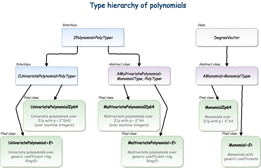
Polynomials
Rings has separate implementation of univariate (dense) and multivariate (sparse) polynomials. Polynomials over \(Z_p\) with \(p < 2^{64}\) are also implemented separately and specifically optimized (coefficients are represented as primitive machine integers instead of generic templatized objects and fast modular arithmetic is used, see Modular arithmetic with machine integers). Below the type hierarchy of polynomial classes is shown:
String representation of polynomials
The first thing about the internal representation of polynomials is that polynomial instances do not store the information about particular string names of variables. Variables are treated just as “the first variable”, “the second variable” and so on without specifying particular names (“x” or “y”). As result, if working with polynomials at the low level, one should manually specify which string names of variables used for parsing/stringifying polynomials. Few illusrtations:
import multivar.MultivariatePolynomial

// when parsing "x" will be considered as the "first variable"
// and "y" as "the second", then in the result the particular
// names "x" and "y" are erased
val poly1 = MultivariatePolynomial.parse("x^2 + x*y", "x", "y")
// parse the same polynomial but using "a" and "b" instead of "x" and "y"
val poly2 = MultivariatePolynomial.parse("a^2 + a*b", "a", "b")
// polynomials are equal (no matter which variable names were used when parsing)
assert(poly1 == poly2)
// degree in the first variable
assert(poly1.degree(0) == 2)
// degree in the second variable
assert(poly1.degree(1) == 1)

// this poly differs from poly2 since now "a" is "the second"
// variable and "b" is "the first"
val poly3 = MultivariatePolynomial.parse("a^2 + a*b", "b", "a")
assert(poly3 != poly2)
// swap the first and the second variables and the result is equal to poly2
assert(poly3.swapVariables(0, 1) == poly2)


// the default toString() will use the default
// variables "x", "y", "z"  (if more variables
// then it will use "x1", "x2", ... , "xN")
// the result will be "x*y + x^2"
println(poly1)
// specify which variable names use for printing
// the result will be "a*b + a^2"
println(poly1.toString("a", "b"))
// the result will be "a*b + b^2"
println(poly1.toString("b", "a"))
// when parsing "x" will be considered as the "first variable"
// and "y" as "the second" => in the result the particular
// names "x" and "y" are erased
MultivariatePolynomial<BigInteger> poly1 = MultivariatePolynomial.parse("x^2 + x*y", "x", "y");
// parse the same polynomial but using "a" and "b" instead of "x" and "y"
MultivariatePolynomial<BigInteger> poly2 = MultivariatePolynomial.parse("a^2 + a*b", "a", "b");
// polynomials are equal (no matter which variable names were used when parsing)
assert poly1.equals(poly2);
// degree in the first variable
assert poly1.degree(0) == 2;
// degree in the second variable
assert poly1.degree(1) == 1;

// this poly differs from poly2 since now "a" is "the second"
// variable and "b" is "the first"
MultivariatePolynomial<BigInteger> poly3 = MultivariatePolynomial.parse("a^2 + a*b", "b", "a");
assert !poly3.equals(poly2);
// swap the first and the second variables and the result is equal to poly2
assert AMultivariatePolynomial.swapVariables(poly3, 0, 1).equals(poly2);


// the default toString() will use the default
// variables "x", "y", "z"  (if more variables
// then it will use "x1", "x2", ... , "xN")
// the result will be "x*y + x^2"
System.out.println(poly1);
// specify which variable names use for printing
// the result will be "a*b + a^2"
System.out.println(poly1.toString("a", "b"));
// the result will be "a*b + b^2"
System.out.println(poly1.toString("b", "a"));
In Java, in order to parse/stringify polynomials, especially over complicated coefficient rings, it is always recomended to use io.Coder (see Input/Output section) instead of factory MultivariatePolynomial.parse(string) methods.
In Scala, information about string names of variables is stored by the ring instance automatically at creation, as well as the appropriate instance of io.Coder which is used internally to parse/stringify ring elements. So in Scala one should parse polynomials with ring(string) and stringify polynomials with ring.stringify(poly). The following example gives a full illustration:
// coefficient ring is GF(17, 3) represented as
// univariate polynomials over "t"
val cfRing = GF(17, 3, "t")

// polynomial ring GF(17, 3)[x, y, z]
implicit val ring = MultivariateRing(cfRing, Array("x", "y", "z"))

// using "x", "y", "z" for polynomial vars and "t" for
// element from GF(17, 3) (that is the eighteenth element
// of GF(17, 3))
val poly = ring("t + x*y - 3*t^9*z^2")

// stringify poly using "x", "y", "z" for polynomial vars
// and "t" for element from GF(17, 3)
println(ring stringify poly)

// one can access underlying coder via `.coder`
// e.g. use it to bind string "p" with polynomial `poly`
ring.coder.bind("p", poly)

val poly2 = ring("x - p^2")
assert(ring.`x` - poly.pow(2) == poly2)

// this is forbidden
// (can't use "a" and "b" instead of "x" and "y")
val polyerr = ring("a^2 + b*c") // <- error!
Tip
In Java, in order to parse polynomial from string as well as to obtain string representation of polynomial it is recomended to use io.Coder (see Input/Output section). In Scala one should parse polynomials with ring(string) and stringify polynomials with ring.stringify(poly).
Polynomial instances and mutability
The second important note about internal implementation of polynomials is that polynomial instances are in general mutable. Methods which may modify the instance are available in Java API, while all mathematical operations applied using Scala DSL (with operators +, - etc.) are not modifier:
val ring = UnivariateRing(Z, "x")
val (p1, p2, p3) = ring("x", "x^2", "x^3")

// this WILL modify p1
p1.add(p2)
// this will NOT modify p2
p2.copy().add(p3)
// this will NOT modify p2
ring.add(p2, p3)
// this will NOT modify p2
p2 + p3
UnivariatePolynomial
        p1 = UnivariatePolynomial.parse("x", Z),
        p2 = UnivariatePolynomial.parse("x^2", Z),
        p3 = UnivariatePolynomial.parse("x^3", Z);

// this WILL modify p1
p1.add(p2);
// this will NOT modify p2
p2.copy().add(p3);
There are strong reasons to use mutable data structures internally for implementation of polynomial algebra. However, it may be confusing when just using the API. So it is always preffered to use ring instance for mathematical operations: use ring.add(a, b) instead of a.add(b) and so on.
Warning
Polynomial instances are mutable. One should call Java API methods on polynomial instances with attention, since they will modify the instance. E.g. a.add(b) will add b directly to the instance a instead of creating a new instance.
Important
When using Rings with Scala it is strongly suggested always to define and use ring instance directly to perform mathematical operations on polynomials. E.g. use ring.add(a, b) or just a + b instead of a.add(b).
The parent interface for all polynomials is IPolynomial<PolyType>. The following example gives a template for implementing generic function which may operate with arbitrary polynomial types:
/**
 * @tparam Poly type of polynomials
 */
def genericFunc[Poly <: IPolynomial[Poly]](poly: Poly): Poly = {
    poly.pow(2) * 3 + poly * 2 + 1
}

// univariate polynomials over Zp64
val uRing = UnivariateRingZp64(17, "x")
println(uRing stringify genericFunc(uRing("1 + 2*x + 3*x^2")))

// multivariate polynomials over Z
val mRing = MultivariateRing(Z, Array("x", "y", "z"))
println(mRing stringify genericFunc(mRing("1 + x + y + z")))
/**
 * @param <Poly> polynomial type
 */
static <Poly extends IPolynomial<Poly>> Poly genericFunc(Poly poly) {
return poly.createOne().add(
        poly.copy().multiply(2),
        polyPow(poly, 2).multiply(3));
}

// univariate polynomials over Zp64
System.out.println(genericFunc(UnivariatePolynomialZ64.create(1, 2, 3).modulus(17)));
// multivariate polynomials over Z
System.out.println(genericFunc(MultivariatePolynomial.parse("1 + x + y + z")));
Note that there is no any specific polynomial ring used in the genericFunc and mathematical operations are delegated to the polynomial instances (plain polynomial addition/multiplication is used). Compare it to the following almost identical example, where the polynomial ring is specified directly and all math operations are delegated to the Ring<E> instance:
/**
  * @tparam Poly type of polynomials
  * @tparam E    type of polynomial coefficients
  */
def genericFuncWithRing[Poly <: IPolynomial[Poly], E](poly: Poly)
    (implicit ring: IPolynomialRing[Poly, E]): Poly = {
  poly.pow(2) * 3 + poly * 2 + 1
}

// univariate polynomials over Zp64
val uRing = UnivariateRingZp64(17, "x")
println(uRing stringify genericFuncWithRing(uRing("1 + 2*x + 3*x^2"))(uRing))

// multivariate polynomials over Z
val mRing = MultivariateRing(Z, Array("x", "y", "z"))
println(mRing stringify genericFuncWithRing(mRing("1 + x + y + z"))(mRing))
/**
 * @param <Poly> polynomial type
 */
static <Poly extends IPolynomial<Poly>> Poly genericFuncWithRing(Poly poly, IPolynomialRing<Poly> ring) {
    return ring.add(
            ring.getOne(),
            ring.multiply(poly, ring.valueOf(2)),
            ring.multiply(ring.pow(poly, 2), ring.valueOf(3)));
}

// univariate polynomials over Zp64
UnivariateRing<UnivariatePolynomialZp64> uRing = UnivariateRingZp64(17);
System.out.println(genericFuncWithRing(uRing.parse("1 + 2*x + 3*x^2"), uRing));

// multivariate polynomials over Z
MultivariateRing<MultivariatePolynomial<BigInteger>> mRing = MultivariateRing(3, Z);
System.out.println(genericFuncWithRing(mRing.parse("1 + x + y + z"), mRing));
While in case of UnivariateRingZp64 or MultivariateRing both genericFunc and genericFuncWithRing give the same result, in the case of e.g. Galois field the results will be different, since mathematical operations in Galois field are performed modulo the irreducible polynomial:
// GF(13^4)
implicit val gf = GF(13, 4, "z")
// some element of GF(13^4)
val poly = gf("1 + z + z^2 + z^3 + z^4").pow(10)

val noRing = genericFunc(poly)
println(noRing)

val withRing = genericFuncWithRing(poly)
println(withRing)

assert(noRing != withRing)
// GF(13^4)
FiniteField<UnivariatePolynomialZp64> gf = GF(13, 4);
// some element of GF(13^4)
UnivariatePolynomialZp64 poly = gf.pow(gf.parse("1 + z + z^2 + z^3 + z^4"), 10);

UnivariatePolynomialZp64 noRing = genericFunc(poly);
System.out.println(noRing);

UnivariatePolynomialZp64 withRing = genericFuncWithRing(poly, gf);
System.out.println(withRing);

assert !noRing.equals(withRing);
Polynomial GCD, factorization and division with remainder
For convenience, the high-level useful methods such as polynomial GCD and factorization are collected in PolynomialMethods class. PolynomialMethods is just a facade which delegates method call to specialized implementation depending on the type of input (univariate or multivariate). The following methods are collected in PolynomialMethods:
FactorSquareFree(poly)
Gives square-free factor decomposition of given polynomial.Factor(poly)
Gives complete factor decomposition of polynomial.PolynomialGCD(a, b, c, ...)
Gives greatest common divisor of given polynomials.divideAndRemainder(dividend, divider)
Gives quotient and remainder of the input.remainder(dividend, divider)
Gives the remainder ofdividendanddivider.coprimeQ(a, b, c, ...)
Tests whether specified polynomials are pairwise coprime.polyPow(poly, exponent)
Gives polynomials in a power of specified exponent.
The examples of polynomial factorization and GCD are given in the below sections and in the Quick Tour.
Univariate polynomials
Rings has two separate implementations of univariate polynomials:
- UnivariatePolynomialZp64 — univariate polynomials over \(Z_p\) with \(p < 2^{64}\). Implementation of UnivariatePolynomialZp64 uses specifically optimized data structure and efficient algorithms for arithmetic in \(Z_p\) (see Modular arithmetic with machine integers).
- UnivariatePolynomial<E> — univariate polynomials over generic coefficient ring Ring<E>.
Internally both implementations use dense data structure (array of coefficients) and Karatsuba’s algrotithm for multiplication (Sec. 8.1 in [GaGe03]). Generic interface IUnivariatePolynomial unifies methods of these two implementations. The following template shows how to write generic function which works with both types of univariate polynomials:
/**
  * @tparam Poly type of univariate polynomials
  */
def genericFunc[Poly <: IUnivariatePolynomial[Poly]](poly: Poly) = ???

/**
  * @tparam Poly type of univariate polynomials
  * @tparam E    type of polynomial coefficients
  */
def genericFuncWithRing[Poly <: IUnivariatePolynomial[Poly], E](poly: Poly)
    (implicit ring: IUnivariateRing[Poly, E]) =  ???
/**
 * @param <Poly> univariate polynomial type
 */
static <Poly extends IUnivariatePolynomial<Poly>>
Poly genericFunc(Poly poly) { return null; }

/**
 * @param <Poly> univariate polynomial type
 */
static <Poly extends IUnivariatePolynomial<Poly>>
Poly genericFuncWithRing(Poly poly, IPolynomialRing<Poly> ring) { return null; }
Univariate division with remainder
There are several algorithms for division with remainder of univariate polynomials implemented in Rings:
UnivariateDivision.divideAndRemainderClassic
Plain divisionUnivariateDivision.pseudoDivideAndRemainder
Plain pseudo division of polynomials over non-fieldsUnivariateDivision.divideAndRemainderFast
Fast division via Newton iterations (Sec. 11 in [GaGe03])
The upper-level method UnivariateDivision.divideAndRemainder switches between plain and fast division depending on the input. The algorithm with Newton iterations allows to precompute Newton inverses for the divider and then use it for divisions by that divider. This allows to achieve considerable performance boost when need to do several divisions with a fixed divider (e.g. for implementation of Galois fields). Examples:
implicit val ring = UnivariateRingZp64(17, "x")
// some random divider
val divider = ring.randomElement()
// some random dividend
val dividend = 1 + 2 * divider + 3 * divider.pow(2)

// quotient and remainder using built-in methods
val (divPlain, remPlain) = dividend /% divider

// precomputed Newton inverses, need to calculate it only once
implicit val invMod = divider.precomputedInverses
// quotient and remainder computed using fast
// algorithm with precomputed Newton inverses
val (divFast, remFast) = dividend /%% divider

// results are the same
assert((divPlain, remPlain) == (divFast, remFast))
UnivariateRing<UnivariatePolynomialZp64> ring = UnivariateRingZp64(17);
// some random divider
UnivariatePolynomialZp64 divider = ring.randomElement();
// some random dividend
UnivariatePolynomialZp64 dividend = ring.add(
        ring.valueOf(1),
        ring.multiply(ring.valueOf(2), divider),
        ring.multiply(ring.valueOf(3), ring.pow(divider, 2)));

// quotient and remainder using built-in methods
UnivariatePolynomialZp64[] divRemPlain
        = UnivariateDivision.divideAndRemainder(dividend, divider, true);

// precomputed Newton inverses, need to calculate it only once
UnivariateDivision.InverseModMonomial<UnivariatePolynomialZp64> invMod
        = UnivariateDivision.fastDivisionPreConditioning(divider);
// quotient and remainder computed using fast
// algorithm with precomputed Newton inverses
UnivariatePolynomialZp64[] divRemFast
        = UnivariateDivision.divideAndRemainderFast(dividend, divider, invMod, true);

// results are the same
assert Arrays.equals(divRemPlain, divRemFast);
Details of implementation can be found in UnivariateDivision.
Univariate GCD
Rings have several algorithms for univariate GCD:
UnivariateGCD.EuclidGCDandUnivariateGCD.ExtedndedEuclidGCD
Euclidean algorithm (and its extended version)UnivariateGCD.HalfGCDandUnivariateGCD.ExtedndedHalfGCD
Half-GCD (and its extended version) (Sec. 11 [GaGe03])UnivariateGCD.SubresultantRemainders
Subresultant sequences (Sec. 7.3 in [GeCL92])UnivariateGCD.ModularGCDandUnivariateGCD.ModularExtendedGCD
Modular GCD (Sec. 6.7 in [GaGe03], small primes version) and modular extended GCD with rational reconstruction (Sec. 6.11 in [GaGe03])
The upper-level method UnivariateGCD.PolynomialGCD switches between Euclidean algorithm and Half-GCD for polynomials in \(F[x]\) where \(F\) is a finite field. For polynomials in \(Z[x]\) and \(Q[x]\) the modular algorithm is used (small primes version). In other cases algorithm with subresultant sequences is used. Examples:
import poly.univar.UnivariateGCD._

// Polynomials over field
val ringZp = UnivariateRingZp64(17, "x")
val a = ringZp("1 + 3*x + 2*x^2")
val b = ringZp("1 - x^2")
// Euclid and Half-GCD algorithms for polynomials over field
assert(EuclidGCD(a, b) == HalfGCD(a, b))
// Extended Euclidean algorithm
val (gcd, s, t) = ExtendedEuclidGCD(a, b) match {case Array(gcd, s, t) => (gcd, s, t)}
assert(a * s + b * t == gcd)
// Extended Half-GCD algorithm
val (gcd1, s1, t1) = ExtendedHalfGCD(a, b) match {case Array(gcd, s, t) => (gcd, s, t)}
assert((gcd1, s1, t1) == (gcd, s, t))


// Polynomials over Z
val ringZ = UnivariateRing(Z, "x")
val aZ = ringZ("1 + 3*x + 2*x^2")
val bZ = ringZ("1 - x^2")
// GCD for polynomials over Z
assert(ModularGCD(aZ, bZ) == ringZ("1 + x"))


// Bivariate polynomials represented as Z[y][x]
val ringXY = UnivariateRing(UnivariateRing(Z, "y"), "x")
val aXY = ringXY("(1 + y) + (1 + y^2)*x + (y - y^2)*x^2")
val bXY = ringXY("(3 + y) + (3 + 2*y + y^2)*x + (3*y - y^2)*x^2")
// Subresultant sequence
val subResultants = SubresultantRemainders(aXY, bXY)
// The GCD
val gcdXY = subResultants.gcd.primitivePart
assert(aXY % gcdXY === 0 && bXY % gcdXY === 0)
// Polynomials over field
UnivariatePolynomialZp64 a = UnivariatePolynomialZ64.create(1, 3, 2).modulus(17);
UnivariatePolynomialZp64 b = UnivariatePolynomialZ64.create(1, 0, -1).modulus(17);
// Euclid and Half-GCD algorithms for polynomials over field
assert EuclidGCD(a, b).equals(HalfGCD(a, b));
// Extended Euclidean algorithm
UnivariatePolynomialZp64[] xgcd = ExtendedEuclidGCD(a, b);
assert a.copy().multiply(xgcd[1]).add(b.copy().multiply(xgcd[2])).equals(xgcd[0]);
// Extended Half-GCD algorithm
UnivariatePolynomialZp64[] xgcd1 = ExtendedHalfGCD(a, b);
assert Arrays.equals(xgcd, xgcd1);


// Polynomials over Z
UnivariatePolynomial<BigInteger> aZ = UnivariatePolynomial.create(1, 3, 2);
UnivariatePolynomial<BigInteger> bZ = UnivariatePolynomial.create(1, 0, -1);
// GCD for polynomials over Z
assert ModularGCD(aZ, bZ).equals(UnivariatePolynomial.create(1, 1));


// Bivariate polynomials represented as Z[y][x]
UnivariateRing<UnivariatePolynomial<UnivariatePolynomial<BigInteger>>>
        ringXY = UnivariateRing(UnivariateRing(Z));
UnivariatePolynomial<UnivariatePolynomial<BigInteger>>
        aXY = ringXY.parse("(1 + y) + (1 + y^2)*x + (y - y^2)*x^2"),
        bXY = ringXY.parse("(3 + y) + (3 + 2*y + y^2)*x + (3*y - y^2)*x^2");
//// Subresultant sequence
PolynomialRemainders<UnivariatePolynomial<UnivariatePolynomial<BigInteger>>>
        subResultants = SubresultantRemainders(aXY, bXY);
// The GCD
UnivariatePolynomial<UnivariatePolynomial<BigInteger>> gcdXY = subResultants.gcd().primitivePart();
assert UnivariateDivision.remainder(aXY, gcdXY, true).isZero();
assert UnivariateDivision.remainder(bXY, gcdXY, true).isZero();
Details of implementation can be found in UnivariateGCD.
Univariate factorization
Implementation of univariate factorization in Rings is distributed over several classes:
UnivariateSquareFreeFactorization
Square-free factorization of univariate polynomials. In the case of zero characteristic Yun’s algorithm is used (Sec. 14.6 in [GaGe03]), otherwise Musser’s algorithm is used (Sec. 8.3 in [GeCL92], [Muss71]).DistinctDegreeFactorization
Distinct-degree factorization. Internally there are several algorithms: plain (Sec. 14.2 in [GaGe03]), adapted version with precomputed \(x\)-powers, and Victor Shoup’s baby-step giant-step algorithm [Shou95]. The upper-level method swithces between these algorithms depending on the input.EqualDegreeFactorization
Equal-degree factorization using Cantor-Zassenhaus algorithm in both odd and even characteristic (Sec. 14.3 in [GaGe03]).UnivariateFactorization
Defines upper-level methods and implements factorization over \(Z\). In the latter case Hensel lifting (combined linear/quadratic) is used to lift factorization modulo some 32-bit prime number to actual factorization over \(Z\) and naive recombination to reconstruct correct factors. Examples:
Univariate factorization is supported for polynomials in \(F[x]\) where \(F\) is either finite field, \(Z\), \(Q\) or other polynomial ring. Examples:
// ring GF(13^5)[x] (coefficient domain is finite field)
val ringF = UnivariateRing(GF(13, 5, "z"), "x")
// some random polynomial composed from some factors
val polyF = ringF.randomElement() * ringF.randomElement() * ringF.randomElement().pow(10)
// perform square-free factorization
println(ringF stringify FactorSquareFree(polyF))
// perform complete factorization
println(ringF stringify Factor(polyF))


// ring Q[x]
val ringQ = UnivariateRing(Q, "x")
// some random polynomial composed from some factors
val polyQ = ringQ.randomElement() * ringQ.randomElement() * ringQ.randomElement().pow(10)
// perform square-free factorization
println(ringQ stringify FactorSquareFree(polyQ))
// perform complete factorization
println(ringQ stringify Factor(polyQ))
// ring GF(13^5)[x] (coefficient domain is finite field)
UnivariateRing<UnivariatePolynomial<UnivariatePolynomialZp64>> ringF = UnivariateRing(GF(13, 5));
// some random polynomial composed from some factors
UnivariatePolynomial<UnivariatePolynomialZp64> polyF = ringF.randomElement().multiply(ringF.randomElement().multiply(polyPow(ringF.randomElement(), 10)));

// perform square-free factorization
System.out.println(FactorSquareFree(polyF));
// perform complete factorization
System.out.println(Factor(polyF));


// ring Q[x]
UnivariateRing<UnivariatePolynomial<Rational<BigInteger>>> ringQ = UnivariateRing(Q);
// some random polynomial composed from some factors
UnivariatePolynomial<Rational<BigInteger>> polyQ = ringQ.randomElement().multiply(ringQ.randomElement().multiply(polyPow(ringQ.randomElement(), 10)));
// perform square-free factorization
System.out.println(FactorSquareFree(polyQ));
// perform complete factorization
System.out.println(Factor(polyQ));
Details of implementation can be found in UnivariateSquareFreeFactorization, DistinctDegreeFactorization, EqualDegreeFactorization and UnivariateFactorization.
Testing irreducibility
Irreducibility test and generation of random irreducible polynomials are availble from IrreduciblePolynomials. For irreducibility testing of polynomials over finite fields the algorithm described in Sec. 14.9 in [GaGe03] is used. Methods implemented in IrreduciblePolynomials are used for construction of arbitrary Galois fields. Examples:
import rings.poly.univar.IrreduciblePolynomials._
val random = new Random()

// random irreducible polynomial in Z/2[x] of degree 10 (UnivariatePolynomialZp64)
val poly1 = randomIrreduciblePolynomial(2, 10, random)
assert(poly1.degree() == 10)
assert(irreducibleQ(poly1))

// random irreducible polynomial in Z/2[x] of degree 10 (UnivariatePolynomial[Integer])
val poly2 = randomIrreduciblePolynomial(Zp(2).theRing, 10, random)
assert(poly2.degree() == 10)
assert(irreducibleQ(poly2))

// random irreducible polynomial in GF(11^15)[x] of degree 10 (this may take few seconds)
val poly3 = randomIrreduciblePolynomial(GF(11, 15).theRing, 10, random)
assert(poly3.degree() == 10)
assert(irreducibleQ(poly3))

// random irreducible polynomial in Z[x] of degree 10
val poly4 = randomIrreduciblePolynomialOverZ(10, random)
assert(poly4.degree() == 10)
assert(irreducibleQ(poly4))
Well44497b random = new Well44497b();

// random irreducible polynomial in Z/2[x] of degree 10
UnivariatePolynomialZp64 poly1 = randomIrreduciblePolynomial(2, 10, random);
assert poly1.degree() == 10;
assert irreducibleQ(poly1);

// random irreducible polynomial in Z/2[x] of degree 10
UnivariatePolynomial<BigInteger> poly2 = randomIrreduciblePolynomial(Zp(2), 10, random);
assert poly2.degree() == 10;
assert irreducibleQ(poly2);

// random irreducible polynomial in GF(11^15)[x] of degree 10 (this may take few seconds)
UnivariatePolynomial<UnivariatePolynomialZp64> poly3 = randomIrreduciblePolynomial(GF(11, 15), 10, random);
assert poly3.degree() == 10;
assert irreducibleQ(poly3);

// random irreducible polynomial in Z[x] of degree 10
UnivariatePolynomial<BigInteger> poly4 = randomIrreduciblePolynomialOverZ(10, random);
assert poly4.degree() == 10;
assert irreducibleQ(poly4);
The details about implementation can be found in IrreduciblePolynomials.
Univariate interpolation
Polynomial interpolation via Newton method can be done in the following way:
import rings.poly.univar.UnivariateInterpolation._

// points
val points = Array(1L, 2L, 3L, 12L)
// values
val values = Array(3L, 2L, 1L, 6L)

// interpolate using Newton method
val result = new InterpolationZp64(Zp64(17))
  .update(points, values)
  .getInterpolatingPolynomial

// result.evaluate(points(i)) = values(i)
assert(points.zipWithIndex.forall { case (point, i) => result.evaluate(point) == values(i) })
// points
long[] points = {1L, 2L, 3L, 12L};
// values
long[] values = {3L, 2L, 1L, 6L};

// interpolate using Newton method
UnivariatePolynomialZp64 result = new InterpolationZp64(Zp64(17))
        .update(points, values)
        .getInterpolatingPolynomial();

// result.evaluate(points(i)) = values(i)
assert IntStream.range(0, points.length).allMatch(i -> result.evaluate(points[i]) == values[i]);
With Scala DSL it is quite easy to implement Lagrange interpolation formula:
/*  Lagrange interpolation formula */
def lagrange[Poly <: IUnivariatePolynomial[Poly], E](points: Seq[E], values: Seq[E])(implicit ring: IUnivariateRing[Poly, E]) = {
  points.indices
    .foldLeft(ring getZero) { case (sum, i) =>
      sum + points.indices
        .filter(_ != i)
        .foldLeft(ring getConstant values(i)) { case (product, j) =>
          implicit val cfRing = ring.cfRing
          val E: E = points(i) - points(j)
          product * (ring.`x` - points(j)) / E
        }
    }
}

import rings.poly.univar.UnivariateInterpolation._

// coefficient ring GF(13, 5)
implicit val cfRing = GF(13, 5, "z")
val z = cfRing("z")
// some points
val points = Array(1 + z, 2 + z, 3 + z, 12 + z)
// some values
val values = Array(3 + z, 2 + z, 1 + z, 6 + z)

// interpolate with Newton iterations
val withNewton = new Interpolation(cfRing)
  .update(points, values)
  .getInterpolatingPolynomial
// interpolate using Lagrange formula
val withLagrange = lagrange(points, values)(UnivariateRing(cfRing, "x"))
// results are the same
assert(withNewton == withLagrange)
Multivariate polynomials
Rings has two separate implementations of multivariate polynomials:
- MultivariatePolynomialZp64 — multivariate polynomials over \(Z_p\) with \(p < 2^{64}\). Implementation of MultivariatePolynomialZp64 uses efficient algorithms for arithmetic in \(Z_p\) (see Modular arithmetic with machine integers)
- MultivariatePolynomial<E> — multivariate polynomials over generic coefficient ring Ring<E>
Internally both implementations use sparse data structure — map (java.util.TreeMap) from degree vectors (DegreeVector) to monomials (AMonomial) . Monomial type is implemented as just a degree vector which additionally holds a coefficient. So in correspondence with the two implementations of multivariate polynomials there are two implementations of monomials:
- MonomialZp64 — monomial that stores machine-number coefficient (
long) and is used by MultivariatePolynomialZp64- Monomial<E> — monomial that stores generic coefficient of type
Eand is used by MultivariatePolynomial<E>
The generic parent class for multivariate polynomials is AMultivariatePolynomial<MonomialType, PolyType>. The following template shows how to write generic function which works with both types of multivariate polynomials:
/**
  * @tparam Monomial    type of monomials
  * @tparam Poly        type of multivariate polynomials
  */
def genericFunc[
        Monomial <: AMonomial[Monomial],
        Poly <: AMultivariatePolynomial[Monomial, Poly]
    ](poly: Poly) = ???

/**
  * @tparam Monomial    type of monomials
  * @tparam Poly        type of multivariate polynomials
  * @tparam Coefficient type of polynomial coefficients
  */
def genericFuncWithRing[
        Monomial <: AMonomial[Monomial],
        Poly <: AMultivariatePolynomial[Monomial, Poly],
        Coefficient
    ](poly: Poly)
     (implicit ring: IMultivariateRing[Monomial, Poly, Coefficient]) = ???

implicit val ring = MultivariateRing(Z, Array("x", "y", "z"))
import ring.{MonomialType, PolyType, CoefficientType}

val poly = ring.randomElement()

// call generic func directly
genericFunc[MonomialType, PolyType, CoefficientType](poly)
genericFuncWithRing[MonomialType, PolyType, CoefficientType](poly)

// define shortcuts
val func = (p: ring.PolyType) =>
    genericFunc[MonomialType, PolyType, CoefficientType](p)
val funcWithRing = (p: ring.PolyType) =>
    genericFuncWithRing[MonomialType, PolyType, CoefficientType](p)(ring)

// call with shortcuts
func(poly)
funcWithRing(poly)
/**
 * @param <Monomial> type of monomials
 * @param <Poly>     type of multivariate polynomials
 */
static <Monomial extends AMonomial<Monomial>,
        Poly extends AMultivariatePolynomial<Monomial, Poly>>
Poly genericFunc(Poly poly) { return null; }

/**
 * @param <Monomial> type of monomials
 * @param <Poly>     type of multivariate polynomials
 */
static <Monomial extends AMonomial<Monomial>,
        Poly extends AMultivariatePolynomial<Monomial, Poly>>
Poly genericFuncWithRing(Poly poly, IPolynomialRing<Poly> ring) { return null; }

// call generic funcs
genericFunc(MultivariatePolynomial.parse("a + b"));

MultivariateRing<MultivariatePolynomial<BigInteger>> ring = MultivariateRing(3, Z);
genericFuncWithRing(ring.parse("a + b"), ring);
Monomial order
Rings uses sparse data structure for multivariate polynomials — a sorted map (java.util.TreeMap) of degree vectors to monomials. Different sort functions of degree vectors correspond to different monomial orders. There are several monomial orders predefined in MonomialOrder:
LEX
Lexicographic monomial order.ALEX
Antilexicographic monomial order.GRLEX
Graded lexicographic monomial order.GREVLEX
Graded reverse lexicographic monomial order.
By default Rings uses GREVLEX order though the monomial order can be changed in many ways. Examples:
import MonomialOrder._

val ring = MultivariateRing(Z, Array("x", "y"), GREVLEX)

// monomials in GREVLEX order
val poly = ring("x + x^2*y^2 + x*y")
assert(poly.ordering == GREVLEX)

// monomials in LEX order
val poly2 = poly.setOrdering(LEX)
assert(poly2.ordering == LEX)

// monomials in GREVLEX order (lhs ordering is used in binary operations)
val add = poly + poly2
assert(add.ordering == GREVLEX)

// monomials in LEX order (lhs ordering is used in binary operations)
val add2 = poly2 + poly
assert(add2.ordering == LEX)
MultivariateRing<MultivariatePolynomial<BigInteger>> ring
        = MultivariateRing(2, Z, MonomialOrder.GREVLEX);

// poly in GREVLEX
MultivariatePolynomial<BigInteger> poly = ring.parse("x + x^2*y^2 + x*y");
assert poly.ordering == MonomialOrder.GREVLEX;

// poly in LEX
MultivariatePolynomial<BigInteger> poly2 = poly.setOrdering(MonomialOrder.LEX);
assert poly2.ordering == MonomialOrder.LEX;

// poly in GREVLEX (ordering of lhs is used)
MultivariatePolynomial<BigInteger> add = ring.add(poly, poly2);
assert add.ordering == MonomialOrder.GREVLEX;

// poly in LEX (ordering of lhs is used)
MultivariatePolynomial<BigInteger> add2 = ring.add(poly2, poly);
assert add2.ordering == MonomialOrder.LEX;
Multivariate division with remainder
Multivariate division with remainder (polynomial reduction) of polynomial \(dividend\) by the array of \(dividers\) gives array of \(quotients\) and \(remainder\) satisfying the following formula:
Examples:
val ring = MultivariateRing(Z, Array("x", "y", "z"), MonomialOrder.LEX)

val dividend = ring("x - x^2*y^2 + 2*x*y + 1 - z*y^2*x^2 + z").pow(3)
val divider1 = ring("x + y")
val divider2 = ring("x + z")
val divider3 = ring("y + z")

{
  val (quot1, quot2, rem) = dividend /%/% (divider1, divider2)
  assert(dividend == divider1 * quot1 + divider2 * quot2 + rem)
}


{
  val (quot1, quot2, quot3, rem) = dividend /%/% (divider1, divider2, divider3)
  assert(dividend == divider1 * quot1 + divider2 * quot2 + divider3 * quot3 + rem)
}
String[] variables = {"x", "y", "z"};
MultivariatePolynomial<BigInteger>
        dividend = MultivariatePolynomial.parse("x - x^2*y^2 + 2*x*y + 1 - z*y^2*x^2 + z", variables),
        divider1 = MultivariatePolynomial.parse("x + y", variables),
        divider2 = MultivariatePolynomial.parse("x + z", variables),
        divider3 = MultivariatePolynomial.parse("y + z", variables);

dividend = polyPow(dividend, 3);

{
    MultivariatePolynomial<BigInteger>[] divRem
            = MultivariateDivision.divideAndRemainder(dividend, divider1, divider2);

    MultivariatePolynomial<BigInteger>
            quot1 = divRem[0], quot2 = divRem[1], rem = divRem[2];

    assert dividend.equals(rem.copy().add(
            quot1.copy().multiply(divider1),
            quot2.copy().multiply(divider2)));
}

{
    MultivariatePolynomial<BigInteger>[] divRem
            = MultivariateDivision.divideAndRemainder(dividend, divider1, divider2, divider3);

    MultivariatePolynomial<BigInteger>
            quot1 = divRem[0], quot2 = divRem[1], quot3 = divRem[2], rem = divRem[3];

    assert dividend.equals(rem.copy().add(
            quot1.copy().multiply(divider1),
            quot2.copy().multiply(divider2),
            quot3.copy().multiply(divider3)));
}
Important
The resulting array of \(quotients\) and \(remainder\) depend on the order of dividers in the array and on the used monomial order. To get a unique result, use Gröbner basis (see Ideals in multivariate polynomial rings).
Details of implementation can be found in MultivariateDivision.
Multivariate GCD
Rings has several algorithms for multivariate GCD:
BrownGCD
Brown’s GCD for multivariate polynomials over finite fields (see [Brow71], Sec 7.4 in [GeCL92], [Yang09]).ZippelGCD
Zippel’s sparse algorithm for multivariate GCD over fields. Works both in case of monic polynomials with fast Vandermonde linear systems (see [Zipp79], [Zipp93]) and in case of non-monic input (LINZIP, see [dKMW05], [Yang09]).ZippelGCDInZ
Zippel’s sparse algorithm for multivariate GCD over Z (see [Zipp79], [Zipp93], [dKMW05]) (the same interpolation techniques as in ZippelGCD is used)..ModularGCDInZ
Standard modular algorithm (small primes) for GCD over Z.KaltofenMonaganSparseModularGCDInGF
Kaltofen’s & Monagan’s generic modular GCD (see [KalM99]) for multivariate polynomials over finite fields with very small cardinality with sparse Zippel’s techniques similar to ZippelGCDInZKaltofenMonaganEEZModularGCDInGF
Kaltofen’s & Monagan’s generic modular GCD (see [KalM99]) for multivariate polynomials over finite fields with very small cardinality with EEZ-GCD used for modular imagesEZGCD
Extended Zassenhaus GCD (EZ-GCD) for multivariate polynomials over finite fields (see Sec. 7.6 in [GeCL92] and [MosY73]).EEZGCD
Enhanced Extended Zassenhaus GCD (EEZ-GCD) for multivariate polynomials over finite fields (see [Wang80]).
The upper-level method MultivariateGCD.PolynomialGCD switches between Zippel-like algorithms and EEZ-GCD based algorithms. The latter are used only on a very dense problems (which occur rarely), while the former are actually used in most cases. In case of finite fields of very small cardinality Kaltofen’s & Monagan’s algorithm is used. Examples:
import rings.poly.multivar.MultivariateGCD._

// some large finite field
val modulus = SmallPrimes.nextPrime(1 << 15)
val ring = MultivariateRingZp64(modulus, Array("x", "y", "z"))

val a = ring("x^2 - x*y + z^5")
val b = ring("x^2 + x*y^7 + x*y*z^2")

val gcd = ring("x + y + z")
val poly1 = a * gcd
val poly2 = b * gcd

// EZGCD in finite field
val ez = EZGCD(poly1, poly2)
assert(ez == gcd)

// EEZGCD in finite field
val eez = EEZGCD[ring.MonomialType, ring.PolyType](poly1, poly2)
assert(eez == gcd)

// ZippelGCD in finite field
val zippel = ZippelGCD(poly1, poly2)
assert(zippel == gcd)

// some very small finite field (Z/2)
val z2 = Zp64(2)
val z2GCD = gcd.setRing(z2)
val z2Poly1 = a.setRing(z2) * z2GCD
val z2Poly2 = b.setRing(z2) * z2GCD

// Kaltofen’s & Monagan’s generic modular GCD
val modGF = ModularGCDInGF(z2Poly1, z2Poly2)
assert(modGF == z2GCD)

// Z
val zGCD = gcd.setRing[IntZ](Z)
val zPoly1 = a.setRing[IntZ](Z) * zGCD
val zPoly2 = b.setRing[IntZ](Z) * zGCD

// Modular GCD in Z with sparse interpolation
val mod = ModularGCD(zPoly1, zPoly2)
assert(mod == zGCD)
// some large finite field
IntegersZp64 zpRing = Zp64(SmallPrimes.nextPrime(1 << 15));
MultivariatePolynomialZp64
        a = MultivariatePolynomialZp64.parse("x^2 - x*y + z^5", zpRing),
        b = MultivariatePolynomialZp64.parse("x^2 + x*y^7 + x*y*z^2", zpRing);

MultivariatePolynomialZp64
        gcd = MultivariatePolynomialZp64.parse("x + y + z", zpRing),
        poly1 = a.copy().multiply(gcd),
        poly2 = b.copy().multiply(gcd);

// EZGCD in finite field
MultivariatePolynomialZp64 ez = EZGCD(poly1, poly2);
assert ez.equals(gcd);

// EEZGCD in finite field
MultivariatePolynomialZp64 eez = EEZGCD(poly1, poly2);
assert eez.equals(gcd);

// ZippelGCD in finite field
MultivariatePolynomialZp64 zippel = ZippelGCD(poly1, poly2);
assert zippel.equals(gcd);

// some very small finite field (Z/2)
IntegersZp64 z2 = Zp64(2);
MultivariatePolynomialZp64
        z2GCD = gcd.setRing(z2),
        z2Poly1 = a.setRing(z2).multiply(z2GCD),
        z2Poly2 = b.setRing(z2).multiply(z2GCD);

// Kaltofen’s & Monagan’s generic modular GCD
MultivariatePolynomialZp64 modGF = ModularGCDInGF(z2Poly1, z2Poly2);
assert modGF.equals(z2GCD);

// Z
MultivariatePolynomial<BigInteger>
        zGCD = gcd.setRing(Z),
        zPoly1 = a.setRing(Z).multiply(zGCD),
        zPoly2 = b.setRing(Z).multiply(zGCD);

// Modular GCD in Z with sparse interpolation
MultivariatePolynomial<BigInteger> mod = ModularGCD(zPoly1, zPoly2);
assert mod.equals(zGCD);
If one need to calculate GCD of more than two polynomials, it is better to do with PolynomialGCD method which uses efficient algorithm for GCD of array of polynomials instead of sequential gcd of each pair of array elements:
val ring = MultivariateRing(Z, Array("x", "y", "z"))
val (rndDegree, rndSize) = (5, 5)

// some random gcd
val gcd = ring.randomElement(rndDegree, rndSize)
// array of random polynomials which have gcd
val polys = (0 until 10).map(_ => ring.randomElement(rndDegree, rndSize) * gcd)

// fast algorithm for array of polynomials will be used
val fastGCD = PolynomialGCD(polys: _*)
// slow step-by-step gcd calculation
val slowGCD = polys.foldLeft(ring.getZero)((p1, p2) => PolynomialGCD(p1, p2))
// result the same
assert(fastGCD == slowGCD)
MultivariateRing<MultivariatePolynomial<BigInteger>> ring = MultivariateRing(3, Z);
int rndDegree = 5, rndSize = 5;

// some random gcd
MultivariatePolynomial<BigInteger> gcd = ring.randomElement(rndDegree, rndSize);
// array of random polynomials which have gcd
MultivariatePolynomial<BigInteger>[] polys = IntStream.range(0, 10)
        .mapToObj(i -> ring.randomElement(rndDegree, rndSize).multiply(gcd))
            .toArray(MultivariatePolynomial[]::new);

// fast algorithm for array of polynomials will be used
MultivariatePolynomial<BigInteger> fastGCD = PolynomialGCD(polys);
// slow step-by-step gcd calculation
MultivariatePolynomial<BigInteger> slowGCD = Arrays.stream(polys)
        .reduce(ring.getZero(), MultivariateGCD::PolynomialGCD);
// result the same
assert fastGCD.equals(slowGCD);
Details of implementation can be found in MultivariateGCD.
Multivariate factorization
Implementation of multivariate factorization in Rings is distributed over two classes:
MultivariateSquareFreeFactorization
Square-free factorization of multivariate polynomials. In the case of zero characteristic Yun’s algorithm is used (Sec. 14.6 in [GaGe03]), otherwise Musser’s algorithm is used (Sec. 8.3 in [GeCL92], [Muss71]).MultivariateFactorization
Implementation of complete factoring algorithms for polynomials over finite fields, \(Z\) and \(Q\). In the case of bivariate polynomials Rings uses fast dense bivariate factorization with naive recombination (see [Bern99], [LeeM13]) (fast irreducibility tests based on Newton polygons are also performed). Factorization algorithm in case of more than two variables is inspired by Kaltofen (see [Kalt85]) and its modified version (see [LeeM13]). Both sparse lifting and fast quasi-dense algorithm due to Bernardin (see [Bern99] and [LeeM13]) are used.
Multivariate factorization is supported for polynomials in \(F[\mathbf{X}]\) where \(F\) is either finite field, \(Z\), \(Q\) or other polynomial ring. Examples:
// ring GF(13^5)[x, y, z] (coefficient domain is finite field)
val ringF = MultivariateRing(GF(13, 5), Array("x", "y", "z"))
// generate random poly of degree 5 and size 5
def randomPolyF = ringF.randomElement(5, 5) + 1

// some random polynomial composed from some factors
val polyF = randomPolyF * randomPolyF * randomPolyF.pow(2)
// perform square-free factorization
println(ringF stringify FactorSquareFree(polyF))
// perform complete factorization
println(ringF stringify Factor(polyF))


// ring Q[x, y, z]
val ringQ = MultivariateRing(Q, Array("x", "y", "z"))
// generate random poly of degree 5 and size 5
def randomPolyQ = ringQ.randomElement(5, 5) + 1

// some random polynomial composed from some factors
val polyQ = randomPolyQ * randomPolyQ * randomPolyQ.pow(2)
// perform square-free factorization
println(ringQ stringify FactorSquareFree(polyQ))
// perform complete factorization
println(ringQ stringify Factor(polyQ))
// ring GF(13^5)[x, y, z] (coefficient domain is finite field)
MultivariateRing<MultivariatePolynomial<UnivariatePolynomialZp64>>
    ringF = MultivariateRing(3, GF(13, 5));

// generate random poly of degree 5 and size 5
Supplier<MultivariatePolynomial<UnivariatePolynomialZp64>> randomPolyF
    = () -> ringF.randomElement(5, 5).increment();

// some random polynomial composed from some factors
MultivariatePolynomial<UnivariatePolynomialZp64> polyF =
    randomPolyF.get().multiply(
            randomPolyF.get(), ringF.pow(randomPolyF.get(), 2));
// perform square-free factorization
System.out.println(FactorSquareFree(polyF));
// perform complete factorization
System.out.println(Factor(polyF));


// ring Q[x, y, z]
MultivariateRing<MultivariatePolynomial<Rational<BigInteger>>> ringQ = MultivariateRing(3, Q);

Supplier<MultivariatePolynomial<Rational<BigInteger>>> randomPolyQ
    = () -> ringQ.randomElement(5, 5).increment();
// some random polynomial composed from some factors
MultivariatePolynomial<Rational<BigInteger>> polyQ =
    randomPolyQ.get().multiply(
            randomPolyQ.get(), ringQ.pow(randomPolyQ.get(), 2));
// perform square-free factorization
System.out.println(FactorSquareFree(polyQ));
// perform complete factorization
System.out.println(Factor(polyQ));
Details of implementation can be found in MultivariateSquareFreeFactorization, HenselLifting and MultivariateFactorization.
Multivariate Interpolation
Multivariate polynomial interpolation via Newton method can be done in the following way:
import rings.poly.multivar.MultivariateInterpolation._

// ring GF(13^6)[x, y, z]
implicit val ring = MultivariateRing(GF(13, 6, "t"), Array("x", "y", "z"))
val (x, y, z) = ring("x", "y", "z")

// coefficient ring GF(13^6)
val cfRing = ring.cfRing
val t = cfRing("t")
// some points for interpolation
val points: Array[ring.CoefficientType] = {
  // hide implicit ring
  val ring: Any = null
  // enable operations in cfRing
  implicit val _ = cfRing
  Array(1 + t, 2 + t, 3 + t, 12 + t)
}

// some values for interpolation
val values = Array(x + y, x.pow(2) + y * t, y.pow(3), x.pow(4) * t + y)

// interpolation polynomial values for variable z
val result = new Interpolation(ring.variable("z"), ring)
  .update(points, values)
  .getInterpolatingPolynomial

assert(points.zipWithIndex.forall { case (point, i) => result("z" -> point) == values(i) })
// ring GF(13^6)[x, y, z]
FiniteField<UnivariatePolynomialZp64> cfRing = GF(13, 6);
MultivariateRing<MultivariatePolynomial<UnivariatePolynomialZp64>>
    ring = MultivariateRing(3, cfRing);

UnivariatePolynomialZp64[] points = {
    cfRing.parse("1 + t"),
    cfRing.parse("2 + t"),
    cfRing.parse("3 + t"),
    cfRing.parse("12 + t")
};

String[] vars = {"x", "y", "z"};
// some values for interpolation
MultivariatePolynomial[] values = {
    ring.parse("x + y", vars),
    ring.parse(" x^2 + (t) * y", vars),
    ring.parse("y^3", vars),
    ring.parse("(t) * x^4 + y", vars)
};

// interpolation polynomial values for variable z
MultivariatePolynomial<UnivariatePolynomialZp64> result =
    new MultivariateInterpolation.Interpolation(2, ring)
            .update(points, values)
            .getInterpolatingPolynomial();

assert IntStream.range(0, points.length)
    .allMatch(i -> result.evaluate(2, points[i]).equals(values[i]));
Ideals in multivariate polynomial rings
The concept of ideal is implemented in the Ideal class which defines basic operations with ideals. Ideal can be created by providing a finite set of polynomial generators. Gröbner basis (see next section) will be computed automatically with respect to specified monomial order. If no any specific monomial order provided, the monomial order of the base ring will be used (in turn, if no any particular order for base ring specified, GREVLEX will be used).
The following methods are available:
| Description | Java method | Scala method |
|---|---|---|
| Get computed Groebner basis | I.getGroebnerBasis() |
I.groebnerBasis |
| Normal form of polynomial | I.normalForm(p) |
I.normalForm(p) or p %% I |
| Ideal membership | I.contains(p) |
I.contains(p) |
| Radical of ideal membership | I.radicalContains(p) |
I.radicalContains(p) |
| Dimension of ideal | I.dimension() |
I.dimension |
| Degree of ideal | I.degree() |
I.degree |
| Union of ideals | I.union(J) |
I union J or I + J or I ∪ J |
| Intersection of ideals | I.intersection(J) |
I intersection J or I ∩ J |
| Multiplication of ideals | I.multiply(J) |
I * J |
| Quotient of ideals | I.quotient(J) |
I :/ J |
| Hilbert-Poincare series | I.hilbertSeries() |
I.hilbertSeries |
| Ideal of leading terms \(LT(I)\) | I.ltIdeal() |
I.ltIdeal |
| Change monomial order | I.changeOrder(newOrder) |
I.changeOrder(newOrder) |
Examples:
implicit val ring = MultivariateRingZp64(17, Array("x", "y", "z"))
val (x, y, z) = ring("x", "y", "z")

// create ideal with two generators using GREVLEX monomial order for underlying Groebner basis
val I = Ideal(ring, Seq(x.pow(2) + y.pow(12) - z, x.pow(2) * z + y.pow(2) - 1), GREVLEX)
// I is proper ideal
assert(I.isProper)

// get computed Groebner basis
val gb = I.groebnerBasis
println(gb)

// check some ideal properties
assert(I.dimension == 1)
assert(I.degree == 36)

// create another ideal with only one generator
val J = Ideal(ring, Seq(x.pow(4) * y.pow(4) + 1), GREVLEX)
// J is principal ideal
assert(J.isPrincipal)
assert(J.dimension == 2)
assert(J.degree == 8)


val union = I union J
// union is zero dimensional ideal
assert(union.dimension == 0)
// change order to LEX (elimination order)
val eliminated = union.changeOrder(LEX)
// system can now be solved easily
println(eliminated)


val intersection = I intersection J
// intersection is still 2-dimensional
assert(intersection.dimension == 2)
// multiplication in this case is equal to intersection
val times = I * J
assert(times == intersection)


// yet another ideal
val K = Ideal(ring, Seq(z * x.pow(4) - z * y.pow(14) + y * z.pow(16), (x + y + z).pow(4)), GREVLEX)
// compute complicated quotient ideal
val quot = (I * J * K) :/ times
assert(quot == K)
MultivariateRing<MultivariatePolynomialZp64> ring = MultivariateRingZp64(3, 17);

// create ideal with two generators using GREVLEX monomial order for underlying Groebner basis
Ideal<MonomialZp64, MultivariatePolynomialZp64> I = Ideal.create(Arrays.asList(
    ring.parse("x^2 + y^12 - z"),
    ring.parse("x^2 * z + y^2 - 1")), GREVLEX);
// I is proper ideal
assert I.isProper();

// get computed Groebner basis
List<MultivariatePolynomialZp64> gb = I.getGroebnerBasis();
System.out.println(gb);

// check some ideal properties
assert I.dimension() == 1;
assert I.degree() == 36;

// create another ideal with only one generator
Ideal<MonomialZp64, MultivariatePolynomialZp64> J = Ideal.create(Arrays.asList(
    ring.parse("x^4 * y^4 + 1")), GREVLEX);
// J is principal ideal
assert J.isPrincipal();
assert J.dimension() == 2;
assert J.degree() == 8;


Ideal<MonomialZp64, MultivariatePolynomialZp64> union = I.union(J);
// union is zero dimensional ideal
assert union.dimension() == 0;
// change order to LEX (elimination order)
Ideal<MonomialZp64, MultivariatePolynomialZp64> eliminated = union.changeOrder(LEX);
// system can now be solved easily
System.out.println(eliminated);


Ideal<MonomialZp64, MultivariatePolynomialZp64> intersection = I.intersection(J);
// intersection is still 2-dimensional
assert intersection.dimension() == 2;
// multiplication in this case is equal to intersection
Ideal<MonomialZp64, MultivariatePolynomialZp64> times = I.multiply(J);
assert times.equals(intersection);


// yet another ideal
Ideal<MonomialZp64, MultivariatePolynomialZp64> K = Ideal.create(Arrays.asList(
    ring.parse("z * x^4 - z * y^14 + y * z^16"),
    ring.pow(ring.parse("x + y + z"), 4)), GREVLEX);
// compute complicated quotient ideal
Ideal<MonomialZp64, MultivariatePolynomialZp64> quot = (I.multiply(J).multiply(K)).quotient(times);
assert quot.equals(K);
The normal form operation is used to contstruct qotient rings. It is equivalent to taking a remainder of multivariate division of polynomial by a Gröbner basis of the ideal. The monomial order used to perform that division is the order which was used to compute Gröbner basis of ideal:
// base ring in LEX order
implicit val ring = MultivariateRing(Q, Array("x", "y", "z", "t"), LEX)
val (x, y, z, t) = ring("x", "y", "z", "t")

// some polynomial in a base ring order (LEX)
val poly = x + (y^2) * z + (z^3) * y * t + (t^4) * z * y
assert(poly.ordering == LEX)

// some ideal with Groebner basis computed in GREVLEX
val idealGrevLex = Ideal(ring,
                         Seq(y * (x^3) + z * (t^3) - 1,
                             x * y - y * z - z * x + (t^3)),
                         GREVLEX)
assert(idealGrevLex.ordering == GREVLEX)

// normal form of poly will be computed with respect to GREVLEX
// then the result will be re-sorted according to the base ring order (LEX)
val nfGrevLex = poly %% idealGrevLex
assert(nfGrevLex.ordering == LEX)

// the same ideal with Groebner basis in LEX order
val idealLex = idealGrevLex.changeOrder(LEX)
assert(idealLex.ordering == LEX)

// normal form of poly will be computed with respect to LEX
val nfLex = poly %% idealLex
assert(nfLex.ordering == LEX)

// Normal forms computed against LEX basis and GREVLEX basis
// are different (although both polynomials are sorted in LEX)
assert(nfGrevLex != nfLex)
// base ring in LEX order
MultivariateRing<MultivariatePolynomial<Rational<BigInteger>>> ring = MultivariateRing(4, Q, LEX);
String[] variables = {"x", "y", "z", "t"};

// some polynomial in a base ring order (LEX)
MultivariatePolynomial<Rational<BigInteger>> poly =
        ring.parse("x + y^2 * z + z^3 * y * t + t^4 * z * y", variables);
assert poly.ordering == LEX;

// some ideal with Groebner basis computed in GREVLEX
Ideal<Monomial<Rational<BigInteger>>, MultivariatePolynomial<Rational<BigInteger>>>
        idealGrevLex = Ideal.create(Arrays.asList(
                    ring.parse("y * x^3 + z * t^3 - 1", variables),
                    ring.parse("x * y - y * z - z * x + t^3", variables)),
                GREVLEX);
assert idealGrevLex.ordering == GREVLEX;

// normal form of poly will be computed with respect to GREVLEX
// then the result will be re-sorted according to the base ring order (LEX)
MultivariatePolynomial<Rational<BigInteger>> nfGrevLex = idealGrevLex.normalForm(poly);
assert nfGrevLex.ordering == LEX;

// the same ideal with Groebner basis in LEX order
Ideal<Monomial<Rational<BigInteger>>, MultivariatePolynomial<Rational<BigInteger>>>
        idealLex = idealGrevLex.changeOrder(LEX);
assert idealLex.ordering == LEX;

// normal form of poly will be computed with respect to LEX
MultivariatePolynomial<Rational<BigInteger>> nfLex = idealLex.normalForm(poly);
assert nfLex.ordering == LEX;

// Normal forms computed against LEX basis and GREVLEX basis
// are different (although both polynomials are sorted in LEX)
assert !nfGrevLex.equals(nfLex);
Important
If the coefficient ring \(R\) of a base ring is not a field, Rings will “effectively” perform all operations with coefficients as in the field of fractions \(Frac(R)\). Thus, in Rings ideals in \(Z[x_1, \dots, x_N]\) are actually treated as ideals in \(Q[x_1, \dots, x_N]\).
Hilbert-Poincare series
The Hilbert-Poincare series of ideal in the \(N\)-variate polynomial ring \(S = R[x_1, \dots, x_N]\) has the following form:
where the last equality is obtained by cancellation of common \((1 - t)\) factors from numerator and denominator. We’ll refer the latter form of Hilbert-Poincare series as reduced form. Dimension and degree of ideal are easily computable from its reduced Hilbert-Poincare series: dimension of ideal equal to the degree of denominator and degree of ideal equal to \(N_2(1)\).
Hilbert series of ideal can be obtained by the I.hilbertSeries() method. The return object has the following properties:
| Description | Java/Scala method |
|---|---|
| Initial numerator \(N_1(t)\) | hps.initialNumerator |
| Reduced numerator \(N_2(t)\) | hps.numerator |
| Dimension of ideal | hps.dimension() |
| Degree of ideal | hps.degree() |
| Hilbert polynomial \(HP(m) \in Q[m]\) | hps.hilbertPolynomial() |
| Integer Hilbert polynomial \(HP_Z(m) = (\mbox{dim} - 1)! \times HP(m)\) | hps.hilbertPolynomialZ() |
Examples:
implicit val ring = MultivariateRingZp64(32003, Array("x", "y", "z"))
val (x, y, z) = ring("x", "y", "z")

// some ideal
val ideal = Ideal(ring, Seq(x.pow(2), y.pow(2), z.pow(2)))
// get Hilbert-Poincare series
val hps = ideal.hilbertSeries

assert(hps.dimension == 0)
assert(hps.degree == 8)

// series numerator
println(hps.initialNumerator)
// reduced series numerator
println(hps.numerator)

// integer Hilbert polynomial
println(hps.hilbertPolynomialZ)
// rational Hilbert polynomial
println(hps.hilbertPolynomial)
MultivariateRing<MultivariatePolynomialZp64> ring = MultivariateRingZp64(3, 32003);
Ideal<MonomialZp64, MultivariatePolynomialZp64> ideal
        = Ideal.create(Arrays.asList(
                    ring.parse("x^2"),
                    ring.parse("y^2"),
                    ring.parse("z^2")));
// get Hilbert-Poincare series
HilbertSeries hps = ideal.hilbertSeries();

assert hps.dimension() == 0;
assert hps.degree() == 8;

// series numerator
System.out.println(hps.initialNumerator);
// reduced series numerator
System.out.println(hps.numerator);

// integer Hilbert polynomial
System.out.println(hps.hilbertPolynomialZ());
// rational Hilbert polynomial
System.out.println(hps.hilbertPolynomial());
Hilbert-Poincare series of ideal is computed with algorithm describerd in [Trav96]. If the ideal \(I\) is represented by its Gröbner basis in graded order or is homoheneous, then Hilbert series of leading terms ideal is computed, otherwise some “easy” graded Gröbner basis is computed first.
Gröbner bases algorithms
Rings uses different algorithms for computing Gröbner bases of ideals depending on monomial order and coefficient ring used. They are the following:
- In all algorithms the Gebauer-Moller installation [GebM88], [BecW93] of Buchberger criteria is used
- Gröbner bases in finite fields for graded orders are computed with the use of Faugere’s F4 algorithm [Faug99] with fast sparse linear algebra [FauL10] and simplification algorithm due to [JouV11]
- Gröbner bases for non graded orders are first computed with respect to some graded order and then the order is changed with the use of Hilbert-driven methods [Trav96] (with optional use of homogenezation-dehomogenezation steps)
- Gröbner bases in \(Z\) (resp. \(Q\)) may either use F4 or Buchbeger algorithms directly or, in some cases, switch to modular algorithm [Arno03] (especially for small number of indeterminates)
- If the Hilbert-Poincare series of ideal is known in advance, Hilbert-driven algorithm [Trav96], [CLOS97] will be used
- If non of the above cases apply, the plain Buchberger algorithm [Buch76], [BecW93], [CLOS97] is used
- Plain Buchberger algorithm may use either normal selection strategy (for graded orders) or sugar strategy (e.g. for lexicographic order) [GMNR88]
There is no any general way to select the best algorithm a priori, so the default choise of the algorithm may not be optimal. For example, in some cases for polynomials over \(Q\) Buchberger or F4 algorithms may be tremendously slow, while modular algorithm is very fast, while in other, no more rare cases, modular algorithm may be dramatically slower than plain Buchberger. So, the general advice for complicated ideals is to try different algorithms when the default method is slow.
All algorithms are available from GroebnerBasis class:
// some ideal in Z[x,y,z] with very simple Groebner basis
String[] vars = {"x", "y", "z"};
MultivariatePolynomial<BigInteger>
        a = parse("8*x^2*y^2 + 5*x*y^3 + 3*x^3*z + x^2*y*z", Z, vars),
        b = parse("x^5 + 2*y^3*z^2 + 13*y^2*z^3 + 5*y*z^4", Z, vars),
        c = parse("8*x^3 + 12*y^3 + x*z^2 + 3", Z, vars),
        d = parse("7*x^2*y^4 + 18*x*y^3*z^2 + y^3*z^3", Z, vars);
List<MultivariatePolynomial<BigInteger>> gens = Arrays.asList(a, b, c, d);


// The default method will use modular algorithm in this case
List<MultivariatePolynomial<BigInteger>> gb = GroebnerBasis.GroebnerBasis(gens, GREVLEX);
// Groebner bases is very simple: <x, z^2, 1 + 4*y^3>
System.out.println(gb);

// Modular algorithm will take few milliseconds
List<MultivariatePolynomial<BigInteger>> mod = GroebnerBasis.ModularGB(gens, GREVLEX);
assert mod.equals(gb);

// F4 algorithm will also take few milliseconds
List<MultivariatePolynomial<BigInteger>> f4 = GroebnerBasis.F4GB(gens, GREVLEX);
assert f4.equals(gb);

// But Buchberger algorithm will take several minutes
// because of intermediate expression swell
List<MultivariatePolynomial<BigInteger>> buch = GroebnerBasis.BuchbergerGB(gens, GREVLEX);
assert buch.equals(gb);